Random Variables and Probability Distributions
LEARNING OBJECTIVES
- To learn the concept of the probability distribution of a discrete random variable.
- To learn the concepts of the mean, variance, and standard deviation of a discrete random variable, and how to compute them.
Probability Distributions
Associated to each possible value  of a discrete random variable
  is the probability
 ") that will take the value in one trial of the experiment.
that will take the value in one trial of the experiment.
Definition
The probability distribution of a discrete random variable is a list of each possible value of together with the probability that takes that value in one trial of the experiment.
The probabilities in the probability distribution of a random variable must satisfy the following two conditions:
1. Each probability must be between o and 1:  \leq 1") .
.
2. The sum of all the probabilities is =1") .
.
EXAMPLE 1
A fair coin is tossed twice. Let be the number of heads that are observed.
a. Construct the probability distribution of .
b. Find the probability that at least one head is observed.
Solution:
a. The possible values that can take are 0,1 , and 2 . Each of these numbers corresponds to an event in the sample space  of equally likely outcomes for this experiment:
  to
to  to
to  , and
, and  to
to  . The probability of each of these events, hence of the corresponding value of , can be found simply by counting, to give
|
0 | 1 | 2 |
|
0.25 | 0.50 | 0.25 |
.
b. "At least one head" is the event  , which is the union of the mutually exclusive events
  and . Thus
=P(1)+P(2)=0.50+0.25=0.75
\end{align*}")
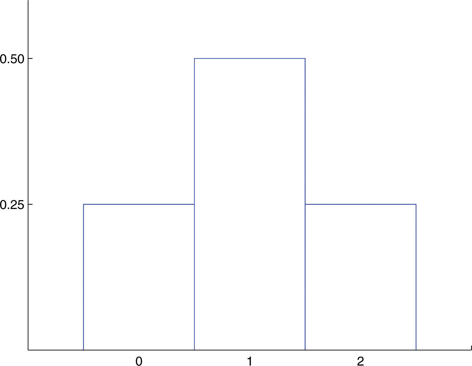
A histogram that graphically illustrates the probability distribution is given in Figure 4.1 "Probability Distribution for Tossing a Fair Coin Twice".
Figure 4.1
Probability Distribution for Tossing a Fair Coin Twice
EXAMPLE 2
A pair of fair dice is rolled. Let denote the sum of the number of dots on the top faces.
a. Construct the probability distribution of .
b. Find ") .
.
c. Find the probability that takes an even value.
Solution:
The sample space of equally likely outcomes is
| 11 | 12 | 13 | 14 | 15 | 16 |
| 21 | 22 | 23 | 24 | 25 | 26 |
| 31 | 32 | 33 | 34 | 35 | 36 |
| 41 | 42 | 43 | 44 | 45 | 46 |
| 51 | 52 | 53 | 54 | 55 | 56 |
| 61 | 62 | 63 | 64 | 65 | 66 |
a. The possible values for are the numbers 2 through 12 . is the event  , so
, so =1 / 36 . X=3") is the event
is the event  , so
, so =2 / 36") . Continuing this way we obtain the table
. Continuing this way we obtain the table
 & \frac{1}{36} & \frac{2}{36} & \frac{3}{36} & \frac{4}{36} & \frac{5}{36} & \frac{6}{36} & \frac{5}{36} & \frac{4}{36} & \frac{3}{36} & \frac{2}{36} & \frac{1}{36}
\end{array}")
This table is the probability distribution of .
b. The event  is the union of the mutually exclusive events
  , and
, and  . Thus
=P(9)+P(10)+P(11)+P(12)=\frac{4}{36}+\frac{3}{36}+\frac{2}{36}+\frac{1}{36}=\frac{10}{36}=0.2 \overline{7}
\end{align*}")
c. Before we immediately jump to the conclusion that the probability that takes an even value must be  , note that takes six different even values but only five different odd values. We compute
 &=P(2)+P(4)+P(6)+P(8)+P(10)+P(12) \\
&=\frac{1}{36}+\frac{3}{36}+\frac{5}{36}+\frac{5}{36}+\frac{3}{36}+\frac{1}{36}=\frac{18}{36}=0.5
\end{aligned}
\end{align*}")
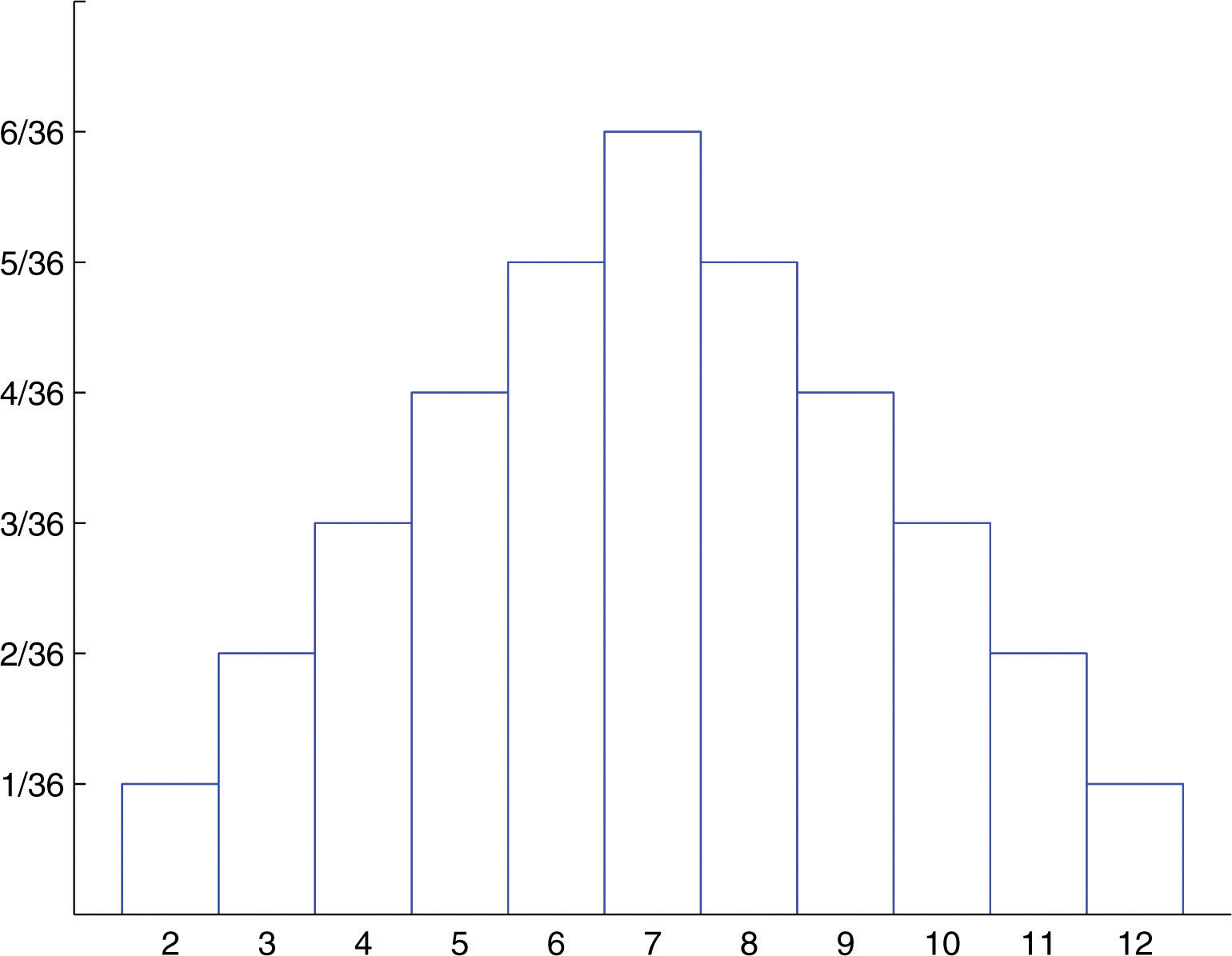
A histogram that graphically illustrates the probability distribution is given in Figure 4.2
"Probability Distribution for Tossing Two Fair Dice".
Figure 4.2
Probability Distribution for Tossing Two Fair Dice