Combinations of Functions
| Site: | Saylor Academy |
| Course: | MA005: Calculus I |
| Book: | Combinations of Functions |
| Printed by: | Guest user |
| Date: | Tuesday, October 22, 2024, 5:35 AM |
Description
Read this section for an introduction to combinations of functions, then work through practice problems 1-9.
Table of contents
- Multiline Definitions of Functions – Putting Pieces Together
- Composition of Functions - Functions of Functions
- Shifting and Stretching Graphs
- Iteration of Functions
- Two Useful Functions: Absolute Value and Greatest Integer
- Absolute Value Function: |x|
- Greatest Integer Function: [x] or INT(x)
- A Really "Holey" Function
- Practice Problem Answers
Multiline Definitions of Functions – Putting Pieces Together
Sometimes a physical or economic situation behaves differently depending on circumstances, and a more complicated function may be needed to describe the situation.
Sales Tax: Some states have different rates of sale tax
depending on the type of item purchased. A "luxury item" may be taxed at 12%, food may have no tax, and all other items may have a 6% tax. We could describe this situation by using a multiline function, a function whose defining
rule consists of several pieces. Which piece of the rule we need to use will depend on what we buy. In this example we could define the tax T on an item which costs x to be
 = \left\{ \begin{array}{lll}0 & \mbox { if
x is the cost of a food}\\ 0.12x & \mbox { if
x is the cost of a luxury item}\\ 0.06x & \mbox { if
x is the cost of any other item} \end{array} \right.")
To find the tax on a $2 can of stew, we would use the first piece of the rule and find that the tax is 0. To find the tax on a $30 pair of earrings, we would use the second piece of the rule and find that the tax is $3.60 . The tax on a $20
book requires using the third rule, and the tax is $1.20 .
Wind Chill Index: The rate at which a person's body loses heat depends on the temperature of the surrounding air and on the speed of the air. You
lose heat more quickly on a windy day than you do on a day with little or no wind. Scientists have experimentally determined this rate of heat loss as a function of temperature and wind speed, and the resulting function is called the Wind
Chill Index, WCI . The WCI is the temperature on a still day (no wind) at which your body would lose heat at the same rate as on the windy day. For example, the WCI value for 30o F air moving at
15 miles per hour is 9o F: your body loses heat as quickly on a 30o F day with a 15 mph wind as it does on a 9o F day with no wind.
If T is the Fahrenheit temperature of the air
and v is the speed of the wind in miles per hour, then the  is a multiline function of the wind speed
  (and of the temperature
  ):
):
 & \mbox { if 4 ≤ v ≤ 45}\\ 1.60T – 55 & \mbox { if v > 45} \end{array} \right.")
The value for a still day ") is just the air temperature. The values for wind speeds
above 45 mph are the same as the value for a wind speed of 45 mph. The values for wind speeds between 4 mph and 45 mph decrease as the wind speeds increase.
is just the air temperature. The values for wind speeds
above 45 mph are the same as the value for a wind speed of 45 mph. The values for wind speeds between 4 mph and 45 mph decrease as the wind speeds increase.
This function depends on two
variables, the temperature and the wind speed. However, if the temperature is constant, then the resulting formula for the will only depend on the speed of the wind. If the air temperature is 30o F
(T = 30), then the formula for the Wind Chill Index is 
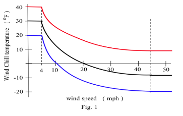
The graphs of the the Wind Chill Indices are shown on Fig. 1 for temperatures of 40o F, 30o F and 20o F . (From UMAP Module 658, Windchill by William Bosch and L.G. Cobb, 1984).
Practice 1: A motel charges $50 per night for a room during the tourist season from June 1 through September 15, and $40 per night otherwise. Define a multiline function which describes these rates.
Example
1: Define  = \left\{ \begin{array}{lll} 2 & \text { if } x < 0\\ 2x & \text { if } 0 ≤ x < 2\\ 1 & \text { if } 2 < x \end{array} \right.")
Evaluate ") ,
, ") ,
, ") ,
, ") and
and ") . Graph
. Graph ") for
for  .
.
Solution: To evaluate the function for different values of  , we must first decide which line of the rule applies.
If
, we must first decide which line of the rule applies.
If  , then we need to use the first line of the rule, and
  = 2") . When
. When  or
or  , we need the second line of the function definition, and then
  = 2(0) = 0") and
and 
= 2(1) = 2") . At
. At  the third line is needed, and
  = 1") . Finally, at
. Finally, at  , none of the lines apply: the second line requires
  and the third line requires
 , so is undefined. The graph of
 ") is given in Fig. 2. Note the "hole" above since is not defined by this rule for
is given in Fig. 2. Note the "hole" above since is not defined by this rule for  .
.
Practice 2: Define
 = \left\{ \begin{array}{llll} x & \text { if } x < –1 \\2 & \text { if } –1 ≤ x < 1 \\ –x & \text { if } 1 < x ≤ 3 \\ 1 & \text { if } 4 < x \end {array} \right.")
Graph ") for
for  and evaluate
 ") ,
, ") ,
, ") ,
, ") ,
, ") ,
, ") ,
, ") ,
, ") ,
, ") and
and ") .
.
Practice 3: Write a multiline function definition for
the function
whose graph is given in Fig. 3 .

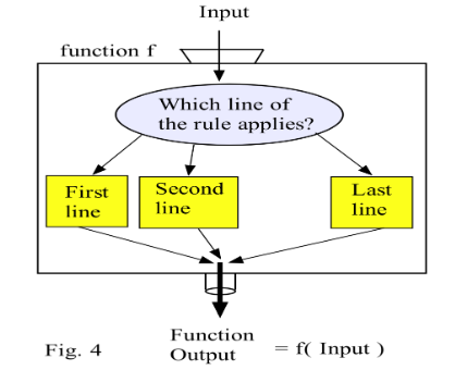
We can think of a multiline function definition as a machine which first examines the input value to decide which line of the function rule to apply (Fig. 4).
Source: Dale Hoffman, https://s3.amazonaws.com/saylordotorg-resources/wwwresources/site/wp-content/uploads/2012/12/MA005-1.4-Combinations-of-Functions.pdf
 This work is licensed under a Creative Commons Attribution 3.0 License.
Composition of Functions - Functions of Functions
Basic functions are often combined with each other to describe more complicated situations. Here we will consider the composition of functions, functions of functions.
Definition: The composite of two functions and  , written
  , is
, is  ≡ f( g(x) )") .
.
The domain of the composite function  = f( g(x) )") consists
of those x–values for which
consists
of those x–values for which ") and
and  )") are both defined - we can evaluate the composition of two functions at a point x only if each step in the composition is defined.
are both defined - we can evaluate the composition of two functions at a point x only if each step in the composition is defined.
If
we think of our functions as machines, then composition is simply
a new machine consisting of an arrangement of the original machines. The composition  of the function machines and shown in
Fig. 5(a) is an arrangement of the machines so that the original input goes into machine , the output from machine becomes the input into machine , and the output from machine is our final output.
The composition of the function machines is only valid if is an allowable input into
of the function machines and shown in
Fig. 5(a) is an arrangement of the machines so that the original input goes into machine , the output from machine becomes the input into machine , and the output from machine is our final output.
The composition of the function machines is only valid if is an allowable input into  is in the domain of
 ") and if is then an allowable input into .
The composition
and if is then an allowable input into .
The composition  involves arranging the machines so the original input goes into , and the output from then becomes the input for (Fig. 5(b) ).

Example 2: For  = x – 2 , g(x) = x^2") , and
, and  = \left\{ \begin{array}{ll} 3x & \mbox { if x < 2 } \\ x – 1 & \mbox { if 2 ≤ x }\end{array} \right.") , evaluate
, evaluate ") ,
, ") ,
, ") and
and ") . Find the equations and domains of
. Find the equations and domains of
") and
and ") .
.
Solution:  = f( g(3) ) = f( 3^2 ) = f( 9 ) = \sqrt{9 – 2} = \sqrt7 ≈ 2.646")
 = g( f(6) ) =
g(\sqrt{6 – 2} ) = g( \sqrt 4 ) = g( 2 ) = 2^2 = 4")
 = f( h(2) ) = f( 2 – 1 ) = f( 1 ) = \sqrt{1 – 2} = \sqrt{–1}") which is undefined
which is undefined
 = h( g(–3) ) = h( 9 ) = 9 – 1 = 8") .
.
 = f( g(x) ) = f( x^2 ) = x^2 – 2") , and the domain of is those x–values for which
, and the domain of is those x–values for which  so the domain
of is all such that
so the domain
of is all such that  or
or  .
.
 = g( f(x) ) = g(\sqrt{ x – 2} ) = { x – 2 }^2 = x – 2") , but we can evaluate the first piece, , of the composition
only if
, but we can evaluate the first piece, , of the composition
only if  = x – 2") is defined, so the domain of is all .
is defined, so the domain of is all .
Practice 4: For  = \frac{x}{x–3}") ,
,  = \sqrt{1+x}") , and
, and  = \left\{ \begin{array}{ll} 2x & \mbox { if x ≤ 1}\\ 5 – x & \mbox { if 1 < x}\end{array} \right.") .
.
Evaluate , ") ,
, ") ,
, ") ,
,
") , and
, and ") . Find the equations for and .
. Find the equations for and .
Shifting and Stretching Graphs
Some compositions are relatively common and easy, and you should recognize the effect of the composition on the graphs of the functions.
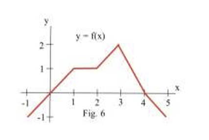
Example 3: Fig. 6 shows the graph of .
Graph (a) ") , (b)
, (b) ") , and
, and  f(x – 1)") .
.
Solution: All of the new graphs are shown below in Fig. 7 .
(a) Adding 2 to all of the values of rigidly shifts the graph of 2 units upward.
(b) Multiplying all of the values of by 3 leaves all of the roots of fixed: if is a root of then  = 0") and
and  = 3(0) = 0") so is also a root of
so is also a root of ") . If is not a root of , then the graph
of
. If is not a root of , then the graph
of ") looks like the graph of stretched vertically by a factor of 3.
looks like the graph of stretched vertically by a factor of 3.
(c) The graph of ") is the graph of rigidly shifted 1 units to the right.
is the graph of rigidly shifted 1 units to the right.

We could also get these results by examining the graph of , creating a table of values for \") and the new functions, and then graphing the new functions.
and the new functions, and then graphing the new functions.
|
|
") |
|
 |
") |
|---|---|---|---|---|---|
| -1 | -1 | 1 | -3 | -2 | ") not definded not definded |
| 0 | 0 | 2 | 0 | -1 |  = -1") |
| 1 | 1 | 3 | 3 | 0 |  = 0") |
| 2 | 1 | 3 | 3 | 1 |  = 1") |
| 3 | 2 | 4 | 6 | 2 |  = 1") |
| 4 | 0 |
2 | 0 | 3 |  = 2") |
| 5 | -1 | 1 | -3 | 4 | ") |
- the graph of
") will be the graph of rigidly shifted up by k units,
will be the graph of rigidly shifted up by k units, - the graph of
") will have the same roots as the graph of and will be the graph of vertically stretched by a factor of
will have the same roots as the graph of and will be the graph of vertically stretched by a factor of  ,
, - the graph of
") will be the graph of rigidly shifted right by units,
will be the graph of rigidly shifted right by units, - the graph of
") will be the graph of rigidly shifted left by units.
will be the graph of rigidly shifted left by units.
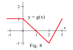
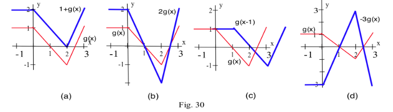
Practice 5: Fig. 8 is the graph of .
Graph (a) ") , (b)
, (b) ") , (c)
, (c) ") and (d)
and (d) ") .
.
Iteration of Functions
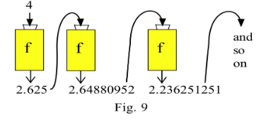
There are applications which feed the output from a function machine back into the same machine as the new input. Each time through the machine is called an iteration of the function.
Example 4: Suppose  = \dfrac{5/x +
x}{2}") , and we start with the input
, and we start with the input  and repeatedly feed the output from back into (Fig. 9). What happens?
Solution:
| Iteration |
Input |
Output |
|---|---|---|
| 1 |
4 |
 =\dfrac{ 5/4 + 4}{2}") = 2.625 = 2.625 |
| 2 |
2.625 |
 ) = \dfrac{5/2.625 + 2.625}{2}") = 2.264880952 = 2.264880952 |
| 3 |
2.264880952 |
 ) )") = 2.236251251 = 2.236251251 |
| 4 |
2.236251251 |
2.236067985 |
| 5 |
2.236067985 |
2.236067977 |
| 6 |
2.236067977 |
2.236067977 |
Once we have obtained the output 2.236067977, we will just keep getting the same output. You might recognize this output value as  . This algorithm always finds
  . If we start with any positive input, the values will eventually get
as close to as we want. Starting with any negative value for the input will eventually get us to
. If we start with any positive input, the values will eventually get
as close to as we want. Starting with any negative value for the input will eventually get us to  . We cannot start with , since 5/0 is undefined.
Practice 6: What happens if we start with
the input value and iterate the function  =\dfrac{9/x + x}{2}") several times? Do you recognize the resulting number? What do you think will happen to the iterates of
several times? Do you recognize the resulting number? What do you think will happen to the iterates of  = \dfrac{A/x + x}{2}") ? (Try several positive values of
? (Try several positive values of
 ).
).
Two Useful Functions: Absolute Value and Greatest Integer
These two functions have useful properties which let us describe situations in which an object abruptly changes direction or jumps from one value to another value.Their graphs will have corners and breaks.
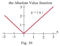
Absolute Value Function: |x|
The absolute value function of a number ,  = | x |") , is the distance between the number and
, is the distance between the number and  . If is greater than or equal to , then
  is simply
  . If is negative, then
  which is positive since
  (negative number) = a positive number. On some calculators and in some computer programming languages, the absolute value
function is represented by
(negative number) = a positive number. On some calculators and in some computer programming languages, the absolute value
function is represented by ") .
.
Definition of  :
:  or
or  .
.
The domain of  = | x |") consists of all real numbers. The range of
consists of all real numbers. The range of  = | x |") consists of all numbers larger than or equal to zero, all non–negative numbers. The graph of
consists of all numbers larger than or equal to zero, all non–negative numbers. The graph of  = | x |") (Fig. 10) has no holes or breaks, but it does have a sharp corner at . The absolute value will be useful later for describing phenomena such as reflected light and bouncing balls which change direction abruptly or whose graphs
have corners.
(Fig. 10) has no holes or breaks, but it does have a sharp corner at . The absolute value will be useful later for describing phenomena such as reflected light and bouncing balls which change direction abruptly or whose graphs
have corners.
The absolute value function has a number of properties which we will use later.
Properties of  : For all real numbers
  and
and  :
:
(a)  .
.  if and
only if
if and
only if  .
.
(b) 
(c) 
Taking the absolute value of a function has an interesting effect on the graph of the function. Since
 , then for any function
 ") we have
we have  | = \left\{ \begin{array}{ll}f(x) & \mbox { if f(x) ≥ 0 }\\–f(x) & \mbox { if f(x) < 0 }\end{array} \right.")
In other words, if  ≥ 0") , then
, then  | = f(x)") so the graph of
so the graph of  |") is the same as the graph of
is the same as the graph of . If f(x) < 0") , then
, then  | = –f(x)") so the graph of is
just the graph of "flipped" about the x–axis, and it lies above the x–axis. The graph of will always be on or above the x–axis.
so the graph of is
just the graph of "flipped" about the x–axis, and it lies above the x–axis. The graph of will always be on or above the x–axis.
Example 5: Fig.
11 shows the graph of . Graph (a) , (b)  |") and (c)
and (c)  |") .
.
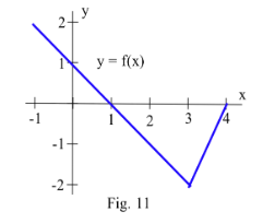
Solution: The graphs are given in Fig. 12. In (b) we shift the graph of  up 1 unit before taking the absolute value. In (c) we take the absolute value before shifting the
graph up 1 unit.
up 1 unit before taking the absolute value. In (c) we take the absolute value before shifting the
graph up 1 unit.

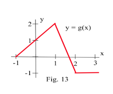
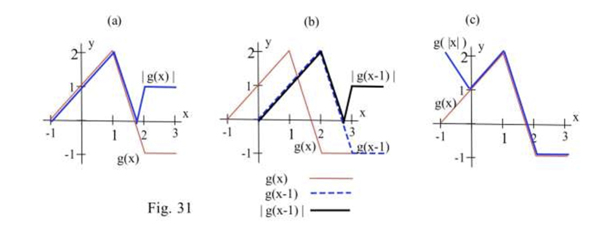
Practice 7: Fig. 13 shows the graph of . Graph (a)  |") , (b)
, (b)  |") , and (c)
, and (c) ") .
.
Greatest Integer Function: [x] or INT(x)
The greatest integer function of a number ![x , y = f(x) = [ x ]](https://dev.saylor.org/filter/tex/pix.php/5db235d9498927a0ddede704119e2906.svg "x , y = f(x) = [ x ]") , is the largest integer which is less than or equal to . The value of
, is the largest integer which is less than or equal to . The value of ![[ x ]](https://dev.saylor.org/filter/tex/pix.php/df937773be1c927baffcc15736629d2a.svg "[ x ]") is always an integer and is always less than or equal to
. For example,
is always an integer and is always less than or equal to
. For example, ![[ 3.2 ] = 3, [ 3.9 ] = 3](https://dev.saylor.org/filter/tex/pix.php/e024814fde8df5b9f6614df9cf5a2114.svg "[ 3.2 ] = 3, [ 3.9 ] = 3") , and
, and ![[ 3 ] = 3](https://dev.saylor.org/filter/tex/pix.php/91ccf63c2dbae7b194cd1699e4ae6e45.svg "[ 3 ] = 3") . If is positive, then truncates (drops the fractional part of ) to get . If is negative,
the situation is different:
. If is positive, then truncates (drops the fractional part of ) to get . If is negative,
the situation is different: ![[ –4.2 ] ≠ –4](https://dev.saylor.org/filter/tex/pix.php/bb74eb0122d7a8df4fb463f986d73023.svg "[ –4.2 ] ≠ –4") since
since  is not less than or equal to
 ![–4.2 : [ –4.2 ] = – 5, [ –4.7 ] = –5](https://dev.saylor.org/filter/tex/pix.php/69aca238f4d0e32a9ac51c2fcd311e65.svg "–4.2 : [ –4.2 ] = – 5, [ –4.7 ] = –5") and
and ![[ –4 ] = –4](https://dev.saylor.org/filter/tex/pix.php/14891780555c768ea3ddccee95f9d84a.svg "[ –4 ] = –4") . On some calculators and in many programming languages the square
brackets
. On some calculators and in many programming languages the square
brackets ![[ \; ]](https://dev.saylor.org/filter/tex/pix.php/d65922b487f7a137b7c7e1f4ef328324.svg "[ \; ]") are used for grouping objects or for lists, and the greatest integer function is represented by
are used for grouping objects or for lists, and the greatest integer function is represented by ") .
.
Definition of : = the largest integer which is less than or equal to
= 
The domain of The ![f(x) = [ x ]](https://dev.saylor.org/filter/tex/pix.php/c6c5b26988f2abe24400749423c864fe.svg "f(x) = [ x ]") is all real numbers. The range of is only the integers. The graph of
is all real numbers. The range of is only the integers. The graph of ![y = f(x) = [ x ]](https://dev.saylor.org/filter/tex/pix.php/b5a13809262735cfa6b41910699447ac.svg "y = f(x) = [ x ]") is shown in Fig. 14. It has a jump break, a step, at each integer
value of , and is called a step function. Between any two consecutive integers, the graph is horizontal with no breaks or holes. The greatest integer function is useful for describing phenomena which change
values abruptly such as postage rates as a function of the weight of the letter ("26¢ for the first ounce and 13¢ additional for each additional half ounce"). It can also be used for functions whose graphs are "square waves" such as the
on and off of a flashing light.
is shown in Fig. 14. It has a jump break, a step, at each integer
value of , and is called a step function. Between any two consecutive integers, the graph is horizontal with no breaks or holes. The greatest integer function is useful for describing phenomena which change
values abruptly such as postage rates as a function of the weight of the letter ("26¢ for the first ounce and 13¢ additional for each additional half ounce"). It can also be used for functions whose graphs are "square waves" such as the
on and off of a flashing light.

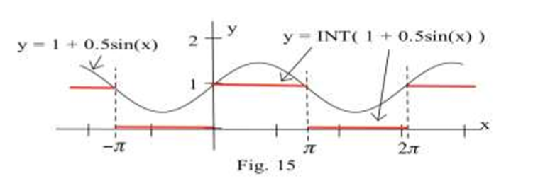
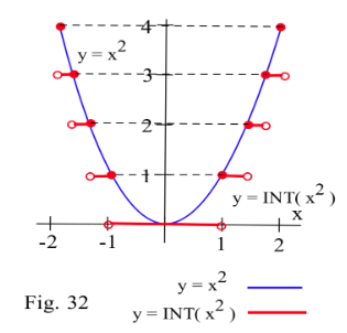
Example 6: Graph  = INT(1 + .5 sin(x) )") .
.
Solution: One way to create this graph is to first graph ") , the thin curve in Fig. 15, and then apply the greatest integer function
to y to get the thicker "square wave" pattern.
, the thin curve in Fig. 15, and then apply the greatest integer function
to y to get the thicker "square wave" pattern.
Practice 8: Sketch the graph of ") for
for  .
.
A Really "Holey" Function
The graph of the greatest integer function has a break or jump at each integer value, but how many breaks can a function have? The next function illustrates just how broken or "holey" the graph of a function can be.
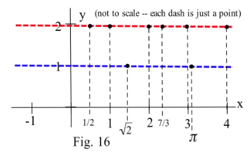
Define
 =\left\{ \begin{array}{ll}
2 & \mbox { if x is a rational number }\\1 & \mbox { if x is an irrational number} \end{array} \right.")
Then  = 2") ,
,  = 2") and
and  = 2") since 3,
5/3 and –2/5 are all rational numbers.
since 3,
5/3 and –2/5 are all rational numbers.  = 1, h(\sqrt 7 ) = 1") , and
, and  = 1") since
since  and
and  are all irrational numbers. These and some
other points are plotted in Fig. 16 .
are all irrational numbers. These and some
other points are plotted in Fig. 16 .
In order to analyze the behavior of ") the following fact about rational and irrational numbers is useful.
the following fact about rational and irrational numbers is useful.
Fact: "Every interval contains both rational and irrational numbers" or, equivalently, "If
and are real numbers and  , then there is
(i) a rational number  between and
 ") , and
, and
(ii) an irrational number  between and
 ") ".
".
The Fact tells us that between any two places where the  = 1") (because is rational) there is a place where
(because is rational) there is a place where ") is 2 because there is an irrational number between any two distinct rational numbers. Similarly,
between any two places where
is 2 because there is an irrational number between any two distinct rational numbers. Similarly,
between any two places where  = 2") (because is irrational) there is a place where because there is a rational number between any two distinct irrational numbers. The graph of
is impossible to actually draw since every two points on the graph are separated by a hole. This is also an example of a function which your computer or calculator can not graph because in general it can not determine whether
an input value of is irrational.
(because is irrational) there is a place where because there is a rational number between any two distinct irrational numbers. The graph of
is impossible to actually draw since every two points on the graph are separated by a hole. This is also an example of a function which your computer or calculator can not graph because in general it can not determine whether
an input value of is irrational.
Example 7: Sketch the graph of  = \left\{ \begin{array}{ll} 2 &\mbox { if x is a rational number }\\ x
& \mbox { if x is an irrational number } \end{array} \right.")
Solution: A sketch of the graph of is shown in Fig. 17 .
When is rational, the graph of looks like the "holey" horizontal line  . When is irrational, the graph of
 ") looks like the "holey"
line
looks like the "holey"
line  .
.

Practice 9: Sketch the graph of  = \left\{ \begin{array}{ll} 2 & \mbox { if x is a rational number }\\ x & \mbox { if x is an irrational number } \end{array}
\right.")
Practice Problem Answers
Practice 1: ") is the cost for one night on date .
is the cost for one night on date .
 = \left\{ \begin{array} {ll} $50 & \text { x is between June 1 and September 15} \\ $40 & \text { if x is any other date } \end{array} \right.")
Practice 2: See Fig. 29

|
|
|---|---|
| -3 | -3 |
| -1 | 2 |
| 0 | 2 |
| 1/2 | 2 |
| 1 | undefined |
|
|
|---|---|
| π/3 |
-π/3 |
| 2 |
-2 |
| 3 |
-3 |
| 4 |
undefined |
| 5 |
1 |
Practice 3:
=\left\{ \begin{array} {lll} 1 & \text { if } x ≤ -1 \\1 -x & \text { if } -1 ≤ x ≤ 1 \\ 2 & \text { if } 1 < x \end{array} \right.")
 = f(2) = 2/–1 = –2") |
 = f(3)") is undefined is undefined |
 = g(4) = \sqrt 5") |
|---|---|---|
 = f(2) = 2/–1 = –2") |
 = f(2) = –2") |
 = f(3)") is undefined is undefined |
 = h(0) = 0") |
 = f(\sqrt{1 + x} ) = ( \sqrt{1+x} )/( \sqrt{1+x} – 3)") , ,  = g(\dfrac{x}{x–3} ) =\sqrt{1 +\dfrac{x}{x–3}}") |
|
Practice 6:  = \dfrac{9/x + x}{2}") .
.
 = \dfrac{9/1 + 1}{2} = 5") ,
,  = \dfrac{9/5 + 5}{2} = 3.4") ,
,  ≈ 3.023529412") ,
,
 ≈ 3.000091554") , and
, and  ≈ 3.000000001") .
.
These values are approaching 3, the square root of 9.
Putting  , then
  = \dfrac{6/x + x}{2}") .
.
 = \dfrac{6/1 + 1}{2} = 3.5") ,
,  = \dfrac{6/3.5 + 3.5}{2} = 2.607142857") ,
,
 ≈ 2.45425636, f(2.45425636) ≈ 2.449494372") ,
,
 ≈ 2.449489743") .
.
 ≈ 2.449489743") (the output is the same as the input for 9 decimal places)
(the output is the same as the input for 9 decimal places)
These values are approaching 2.449489743, the square root of 6.
For any positive value , the iterates of  =\dfrac{A/x+x}{2}") (starting with any positive ) will approach .
(starting with any positive ) will approach .
Practice 7: Fig. 31 shows some of the intermediate steps and final graphs.
Practice 8: Fig. 32 shows the graph of  and the graph (thicker) of .
Practice 9: Fig. 33 shows the "holey" graph of with a hole at each rational value of and the "holey" graph of ") with a hole at each irrational value of . Together they form the graph of
with a hole at each irrational value of . Together they form the graph of ") .
.
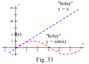
(This is a very crude image since we can't really see the individual holes which have zero width).