Areas, Integrals, and Antiderivatives
| Site: | Saylor Academy |
| Course: | MA005: Calculus I |
| Book: | Areas, Integrals, and Antiderivatives |
| Printed by: | Guest user |
| Date: | Tuesday, October 22, 2024, 3:24 AM |
Description
Read this section to learn about the relationship among areas, integrals, and antiderivatives. Work through practice problems 1-5.
Areas, Integrals, and Antiderivatives
This section explores properties of functions defined as areas and examines some of the connections among areas, integrals and antiderivatives. In order to focus on the geometric meaning and connections, all of the functions in this section are nonnegative, but the results are generalized in the next section and proved true for all continuous functions. This section also introduces examples to illustrate how areas, integrals and antiderivatives can be used.
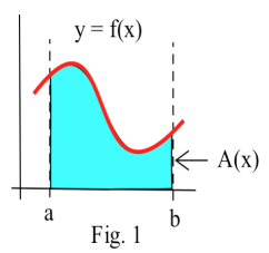
When  is a continuous, nonnegative function, then the "area function"
=\int_{\mathrm{a}}^{x} \mathrm{f}(t) \mathrm{d} \mathrm{t}") represents the area between the graph of , the t–axis, and between the vertical lines at
represents the area between the graph of , the t–axis, and between the vertical lines at  and
and  (Fig. 1), and the derivative of
 ") represents the rate of change (growth) of . Examples 2 and 3 of Section 4.3 showed that for
some functions f, the derivative of was equal to so was an antiderivative of . The next theorem says the result is true for every continuous, nonnegative function .
represents the rate of change (growth) of . Examples 2 and 3 of Section 4.3 showed that for
some functions f, the derivative of was equal to so was an antiderivative of . The next theorem says the result is true for every continuous, nonnegative function .
The Area Function is an Antiderivative
If is a continuous nonnegative function,  and
and =\int_{\mathrm{a}}^{x} \mathrm{f}(t) \mathrm{dt}") .
.
then  \mathrm{dt}\right)=\frac{\mathrm{d}}{\mathrm{dx}} \mathrm{A}(x)=\mathrm{f}(x)") , so is an antiderivative of
, so is an antiderivative of ") .
.
This result relating integrals and antiderivatives is a special case (for nonnegative functions ) of the
Fundamental Theorem of Calculus (Part 1) which is proved in Section 4.5 . This result is important for
two reasons:
(i) it says that a large collection of functions have antiderivatives, and
(ii) it leads to an easy way of exactly evaluating definite integrals.
Example 1: =\int_{1}^{x} \mathrm{f}(t) \mathrm{d} \mathrm{t}") for the function
for the function ") shown in Fig. 2.
shown in Fig. 2.
Estimate the values of and ") for
for  and
and  and use these values to sketch the graph of
 ") .
.
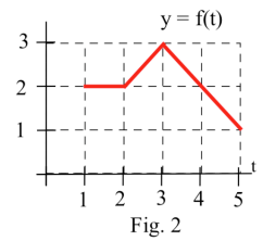
Solution: Dividing the region into squares and triangles, it is easy to see that =2, \mathrm{~A}(3)=4.5, \mathrm{~A}(4)=7") and
and =8.5") . Since
. Since =f(x)") , we
know that
, we
know that =f(2)=2, A^{\prime}(3)=f(3)=3, A^{\prime}(4)=f(4)=2") and
and =f(5)=1") . The graph of
. The graph of ") is shown in Fig. 3.
is shown in Fig. 3.
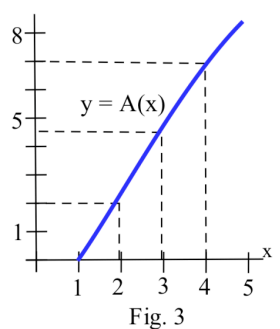
It is important to recognize that f is not differentiable at  and
and  .
However, the values of
.
However, the values of  change smoothly near 2 and 3, and the function is differentiable at those points and at every other point from 1 to 5. Also,
=-1") (
( is clearly decreasing near
  ), but
 =f(4)=2") is positive
(the area is growing even though f is getting smaller).
is positive
(the area is growing even though f is getting smaller).
Practice 1: ") is the area bounded by the horizontal axis, vertical lines at
is the area bounded by the horizontal axis, vertical lines at  and
and  , and the graph of shown in Fig. 4. Estimate the values of and
 ") for
for  and .
and .

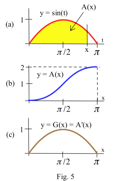
Example 2: Let =\frac{\mathrm{d}}{\mathrm{dx}}\left(\int_{0}^{x} \sin (t) \mathrm{dt}\right)") . Evaluate
. Evaluate ") for
for  .
.
Solution: Fig. 5(a) shows the graph of =\int_{0}^{x} \sin (t) \mathrm{dt}") , and is the derivative of
, and is the derivative of ") . By the theorem,
. By the theorem, =\sin (x)") so
so =\sin (\pi / 4) \approx .707, \mathrm{~A}^{\prime}(\pi / 2)=\sin (\pi / 2)=1") , and
, and =\sin (3 \pi / 4) \approx .707") . Fig. 5(b) shows the graph of and 5(c) is the graph of
. Fig. 5(b) shows the graph of and 5(c) is the graph of =\mathrm{G}(\mathrm{x})") .
.
Source: Dale Hoffman, https://s3.amazonaws.com/saylordotorg-resources/wwwresources/site/wp-content/uploads/2012/12/MA005-5.5-Areas-Integrals-Antiderivatives.pdf This work is licensed under a Creative Commons Attribution 3.0 License.
Using Antiderivatives to Evaluate
Now we can put the ideas of areas and antiderivatives together to get a way of evaluating definite integrals that is exact and often easy.
If , =\int_{\mathrm{a}}^{\mathrm{a}} \mathrm{f}(t) \mathrm{dt}=0, \mathrm{~A}(\mathrm{~b})=\int_{\mathrm{a}}^{\mathrm{b}} \mathrm{f}(t) \mathrm{dt}") and is an antiderivative of ,
and is an antiderivative of , =\mathrm{f}(\mathrm{x})") .
.
We also know that if ") is any antiderivative of , then and have the same derivative so and are "parallel" and differ by a constant,
is any antiderivative of , then and have the same derivative so and are "parallel" and differ by a constant, =A(x)+C") for all
for all  .
.
Then -\mathrm{F}(\mathrm{a})=\{\mathrm{A}(\mathrm{b})+\mathrm{C}\}-\{\mathrm{A}(\mathrm{a})+\mathrm{C}\}=\mathrm{A}(\mathrm{b})-\mathrm{A}(\mathrm{a})=\int_{\mathrm{a}}^{\mathrm{b}} \mathrm{f}(t) \mathrm{dt}-\int_{\mathrm{a}}^{\mathrm{a}} \mathrm{f}(t) \mathrm{dt}=\int_{\mathrm{a}}^{\mathrm{b}} \mathrm{f}(t) \mathrm{dt}") .
.
To evaluate a definite integral  \mathrm{dt}") , we can find any antiderivative
, we can find any antiderivative  of and evaluate
 -\mathrm{F}(\mathrm{a})") .
.
This result is a special case of Part 2 of the Fundamental Theorem of Calculus, and it will be used hundreds of times in the next several chapters. The Fundamental Theorem is stated and proved in Section 4.5.
Antiderivatives and Definite Integrals
If is a continuous, nonnegative function and and is any antiderivative of =\mathrm{f}(x)\right)") on the interval
on the interval ![[a,b]](https://dev.saylor.org/filter/tex/pix.php/2c3d331bc98b44e71cb2aae9edadca7e.svg "[a,b]") ,
,
then  \mathrm{dx}=\mathbf{F}(\mathrm{b})-\mathrm{F}(\mathrm{a})")
The problem of finding the exact value of a definite integral reduces to finding some (any) antiderivative of the integrand and then evaluating =\mathrm{F}(\mathrm{a})") . Even finding one antiderivative can be difficult, and, for now, we will stick to functions which have easy antiderivatives. Later we will explore some methods for finding antiderivatives of more difficult functions.
. Even finding one antiderivative can be difficult, and, for now, we will stick to functions which have easy antiderivatives. Later we will explore some methods for finding antiderivatives of more difficult functions.
The evaluation is represented by the symbol \right|_{a} ^{b}") .
.
Example 3: Evaluate  in two ways:
By sketching the graph of  and geometrically finding the area.
By finding an antiderivative of of and evaluating -\mathrm{F}(1)") .
.
Solution:
(i) The graph of is shown in Fig. 6, and the shaded region has area 4.
(ii) One antiderivative of is =\frac{1}{2} x^{2}") (check that
(check that =x") ), and
), and \right|_{1} ^{3}=\mathrm{F}(3)-\mathrm{F}(1)=\frac{1}{2}\left(3^{2}\right)-\frac{1}{2}\left(1^{2}\right)=\frac{9}{2}-\frac{1}{2}=4") which agrees with (i).
which agrees with (i).
If someone chose another antiderivative of , say =\frac{1}{2} x^{2}+7") ( check that
( check that =x") ), then
), then \right|_{1} ^{3}=\mathrm{F}(3)-\mathrm{F}(1)=\left\{\frac{1}{2}\left(3^{2}\right)+7\right\}-\left\{\frac{1}{2}\left(1^{2}\right)+7\right\}=\frac{23}{2}-\frac{15}{2}=4") . No matter which antiderivative is chosen, equals
. No matter which antiderivative is chosen, equals  .
.

Practice 2: Evaluate  \mathrm{d} x") in the two ways of the previous example.
in the two ways of the previous example.
This antiderivative method is an extremely powerful way to evaluate some definite integrals, and it is used often. However, it can only be used to evaluate a definite integral of a function defined by a formula.
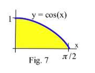
Example 4: Find the area between the graph of the cosine and the horizontal axis for between  and
and  .
.
Solution: The area we want (Fig. 7) is  \mathrm{d} \mathrm{x}") so we need an antiderivative of
so we need an antiderivative of =\cos (x)") .
.
=\sin (x)") is one antiderivative of
is one antiderivative of ") . (Check that
. (Check that ) =\cos (x)") ). Then
). Then  \mathrm{dx}=\left.\sin (x)\right|_{0} ^{\pi / 2}=\sin (\pi / 2)-\sin (0)=1-0=1") .
.
Practice 3: Find the area between the graph of  and the horizontal axis for between 1 and 2.
Integrals, Antiderivatives, and Applications
The antiderivative method of evaluating definite integrals can also be used when we need to find an "area", and it is useful for solving applied problems.
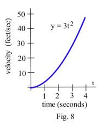
Example 5: A robot has been programmed so that when it starts to move, its
velocity after  seconds will be
  feet/second.
(a) How far will the robot travel during its first 4 seconds of movement?
(b) How far will the robot travel during its next 4 seconds of movement?
(c) How many seconds before the robot is 729 feet from its starting place?
Solution:
(a) The distance during the first 4 seconds will be the area under
the graph (Fig. 8) of velocity , =t") from
from  to
to  , and that
area is the definite integral
, and that
area is the definite integral  . An antiderivative of
 ^{3}-(0)^{3}=64") feet.
feet.
(b) ^{3}-(4)^{3}=512-64=448") feet.
feet.
(c) This part is different from the other two parts. Here we are told the lower integration endpoint, , and the total distance, 729 feet, and we are asked to find the upper endpoint. Calling the upper endpoint  , we know that
 ![729=\int_{0}^{\mathrm{T}} 3 t^{2} \mathrm{dt}=\left.t^{3}\right|_{0} ^{\mathrm{T}}=(\mathrm{T})^{3}-(0)^{3}=\mathrm{T}^{3}, \text { so } \mathrm{T}=\sqrt[3]{729}=9](https://dev.saylor.org/filter/tex/pix.php/ee50fdff8e116f4bfed88f1c8898bb31.svg "729=\int_{0}^{\mathrm{T}} 3 t^{2} \mathrm{dt}=\left.t^{3}\right|_{0} ^{\mathrm{T}}=(\mathrm{T})^{3}-(0)^{3}=\mathrm{T}^{3}, \text { so } \mathrm{T}=\sqrt[3]{729}=9") seconds.
seconds.
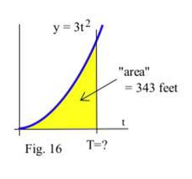
Practice 4: (a) How far will the robot move between  second and
  seconds?
(b) How many seconds before the robot is 343 feet from its starting place?
seconds?
(b) How many seconds before the robot is 343 feet from its starting place?
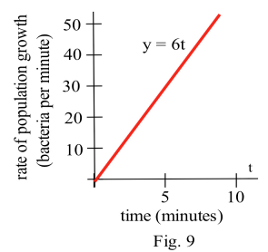
Example 6: Suppose that minutes after putting 1000 bacteria on a Petri plate the rate of growth of the population is 6t bacteria per minute. (a) How many new bacteria are added to the population during the first 7 minutes? (b) What is the total
population after 7 minutes? (c) When will the total population be 2200 bacteria?
Solution:
(a) The number of new bacteria is the area under the rate of growth graph (Fig. 9), and one antiderivative of  is (check that
 =6 t") ) so new bacteria =
) so new bacteria = ^{2}-3(0)^{2}=147") .
.
(b) The new population = {old population} + {new bacteria} = 1000 + 147 = 1147 bacteria
(c) If the total population is 2200 bacteria, then there are 2200 – 1000 = 1200 new bacteria, and we need to find the time T needed for that many new bacteria to occur.
1200 new bacteria = ^{2}-3(0)^{2}=3 \mathrm{~T}^{2} \text { so } \mathrm{T}^{2}=400") and
and  minutes. After 20 minutes, the total bacteria population will be 1000 + 1200 = 2200.
Practice 5: (a) How many new bacteria will be added to the population between and  minutes? (b) When will the total population be 2875 bacteria? (Hint: How many are new?)
Practice Answers
Practice 1: =2.5, \mathrm{~B}(2)=5, \mathrm{~B}(3)=8.5, \mathrm{~B}(4)=12, \mathrm{~B}(5)=14.5")
=\int_{0}^{\mathrm{x}} \mathrm{f}(\mathrm{t}) \mathrm{dt}") so
so =\frac{d}{d x}\left(\int_{0}^{x} f(t) d t\right)=f(x)") (by The Area Function is an Antiderivative
theorem): then
(by The Area Function is an Antiderivative
theorem): then =f(1)=2, B^{\prime}(2)=f(2)=3, B^{\prime}(3)=4, B^{\prime}(4)=3 \text {, }") and
and =2") .
.
Practice 2:
(a) As an area,  is the area of the triangular region between
  and the x– axis for
 (height })=\frac{1}{2}(2)(2)=2") .
.
(b) =\frac{x^{2}}{2}-x") is an antiderivative of
is an antiderivative of =x-1") so
area =
so
area = -\mathrm{F}(1)=\left(\frac{9}{2}-3\right)-\left(\frac{1}{2}-1\right)=2
\end{aligned}") .
.
Practice 3: Area =  .
.
Practice 4:
(a) distance =  = feet.
(b) In this problem we know the starting point is  , and the total distance ("area") is 343 feet. Our problem is to find the time (Fig. 16) so
  .
.
 so
so 
Practice 5:
(a) number of new bacteria =  .
.
(b) We know the total new population ("area" in Fig. 17) is
2875 – 1000 = 1875 so  so
so 
