The Mean Value Theorem and Its Consequences
| Site: | Saylor Academy |
| Course: | MA005: Calculus I |
| Book: | The Mean Value Theorem and Its Consequences |
| Printed by: | Guest user |
| Date: | Tuesday, October 22, 2024, 12:38 AM |
Description
Read this section to learn about the Mean Value Theorem and its consequences. Work through practice problems 1-3.
Introduction
If you averaged 30 miles per hour during a trip, then at some instant during the trip you were traveling exactly 30 miles per hour.
That relatively obvious statement is the Mean Value Theorem as it applies to a particular trip. It may seem strange that such a simple statement would be important or useful to anyone, but the Mean Value Theorem is important and some of its consequences are very useful for people in a variety of areas. Many of the results in the rest of this chapter depend on the Mean Value Theorem, and one of the corollaries of the Mean Value Theorem will be used every time we calculate an "integral" in later chapters. A truly delightful aspect of mathematics is that an idea as simple and obvious as the Mean Value Theorem can be so powerful.
Before we state and prove the Mean Value Theorem and examine some of its consequences, we will consider a simplified version called Rolle's Theorem.
Source: Dale Hoffman, https://s3.amazonaws.com/saylordotorg-resources/wwwresources/site/wp-content/uploads/2012/12/MA005-4.2-Mean-Value-Theorem.pdf This work is licensed under a Creative Commons Attribution 3.0 License.
Rolle's Theorem
Suppose we pick any two points on the  -axis and think about all of the differentiable functions which go through those two points (Fig. 1).
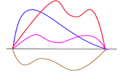
Fig. 1
Since our functions are differentiable, they must be continuous and their graphs can not have any holes or breaks. Also, since these functions are differentiable, their derivatives are defined everywhere between our two points and their graphs can not have any "corners" or vertical tangents. The graphs of the functions in Fig. 1 can still have all sorts of shapes, and it may seem unlikely that they have any common properties other than the ones we have stated, but Michel Rolle found one. He noticed that every one of these functions has one or more points where the tangent line is horizontal (Fig. 2), and this result is named after him.
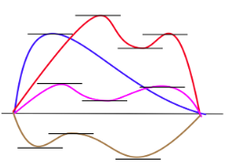
Fig. 2
Rolle's Theorem: If =\mathrm{f}(\mathrm{b})") , and
, and ") is continuous for
is continuous for  and differentiable for
  ,
then there is at least one number
,
then there is at least one number  , between
  and
and  , so that
 =0") .
.
Proof: We consider two cases: when =f(a)") for all in
for all in ") and when
and when  \neq f(a)") for some in .
for some in .
Case I, =\mathrm{f}(\mathrm{a})") for all
for all  in
in ") : If for all between
: If for all between  and
and  , then
 is a horizontal line segment and
 =0") for all values of
for all values of  strictly between and .
Case II, for some in : Since  is continuous on the closed interval
 ![[a, b]](https://dev.saylor.org/filter/tex/pix.php/022022f289db140169cd9514f74ee648.svg "[a, b]") , we know from the Extreme Value Theorem that must have a maximum value in the closed interval
, we know from the Extreme Value Theorem that must have a maximum value in the closed interval ![[\mathrm{a},
\mathrm{b}]](https://dev.saylor.org/filter/tex/pix.php/a927374d960e37867788a825adf599b0.svg "[\mathrm{a},
\mathrm{b}]") and a minimum value in the interval.
and a minimum value in the interval.
If >f(a)") for some value of in , then the maximum of must occur at some value strictly between and
for some value of in , then the maximum of must occur at some value strictly between and  . (Why can't the maximum be at or ?) Since
 ") is a local maximum of ,
then is a critical number of and or
is a local maximum of ,
then is a critical number of and or ") is undefined. But is differentiable at all between and , so the only possibility left is that .
is undefined. But is differentiable at all between and , so the only possibility left is that .
If  < f(a)") for some value of in , then has a minimum at some value
for some value of in , then has a minimum at some value  strictly between a and , and .
In either case, there is at least one value of between and so that .
Example 1: Show that =x^{3}-6 x^{2}+9 x+2") satisfies the hypotheses of Rolle's Theorem on the interval
satisfies the hypotheses of Rolle's Theorem on the interval ![[0,3]](https://dev.saylor.org/filter/tex/pix.php/ed9c05fe24c0f49f5d73f494a921e0c4.svg "[0,3]") and find the value of which the theorem says exists.
and find the value of which the theorem says exists.
Solution: is a polynomial so it is continuous and differentiable everywhere. =2") and
and =2") .
. =3 x^{2}-12 x+9=3(x-1)(x-3)") so
so =0") at
at  and
and  .
.
The value  is between
  and . Fig. 3 shows the graph of .
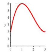
Fig. 3
Practice 1: Find the value(s) of c for Rolle's Theorem for the functions in Fig. 4.
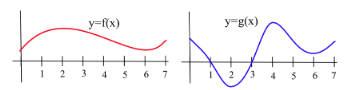
Fig. 4
The Mean Value Theorem
Geometrically, the Mean Value Theorem is a "tilted" version of Rolle's Theorem (Fig. 5). In each theorem we conclude that there is a number so that the slope of the tangent line to at  is the same
as the slope of the line connecting the two ends of the graph of on the interval
is the same
as the slope of the line connecting the two ends of the graph of on the interval ![[\mathrm{a}, \mathrm{b}]](https://dev.saylor.org/filter/tex/pix.php/8c664cf317cce5e2938fe497724bae01.svg "[\mathrm{a}, \mathrm{b}]") . In Rolle's Theorem, the two ends of the graph of are at the same height, ,
so the slope of the line connecting the ends is zero. In the Mean Value Theorem, the two ends of the graph of do not have to be at the same height so the line through the two ends does not have to have a slope of zero.
. In Rolle's Theorem, the two ends of the graph of are at the same height, ,
so the slope of the line connecting the ends is zero. In the Mean Value Theorem, the two ends of the graph of do not have to be at the same height so the line through the two ends does not have to have a slope of zero.
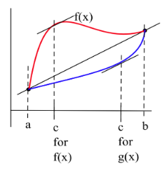
Fig. 5
Mean Value Theorem: If ") is continuous for
is continuous for  and differentiable for
  ,
,
then there is at least one number , between and , so the tangent line at is parallel to the secant line through the points )") and
and ): f^{\prime}(c)=\frac{f(b)-f(a)}{b-a}") .
.
Proof: The proof of the Mean Value Theorem uses a tactic common in mathematics: introduce a new function which satisfies the hypotheses of some theorem we already know and then use the conclusion of that previously proven theorem. For the Mean Value Theorem
we introduce a new function, ") , which satisfies the hypotheses of Rolle's Theorem. Then we can be certain that the conclusion of Rolle's Theorem is true for , and the Mean Value Theorem for
follows from the conclusion of Rolle's Theorem for
, which satisfies the hypotheses of Rolle's Theorem. Then we can be certain that the conclusion of Rolle's Theorem is true for , and the Mean Value Theorem for
follows from the conclusion of Rolle's Theorem for  .
.
First, let ") be the straight line through the ends
be the straight line through the ends )") and
and )") of the graph of . The function
of the graph of . The function  goes through the point
 )") so
so =\mathrm{f}(\mathrm{a})") . Similarly,
. Similarly, =\mathrm{f}(\mathrm{b})") . The slope of the linear function
. The slope of the linear function  is
is -f(a)}{b-a}") so
so =\frac{f(b)-f(a)}{b-a}") for all between and , and is continuous and differentiable. (The formula for is
for all between and , and is continuous and differentiable. (The formula for is =\mathrm{f}(\mathrm{a})+\mathrm{m}(\mathrm{x}-\mathrm{a})") with
with -\mathrm{f}(\mathrm{a}))
/(\mathrm{b}-\mathrm{a})") .)
.)
Define =f(x)-g(x)") for (Fig. 6). The function
for (Fig. 6). The function  satisfies the hypotheses of Rolle's theorem:
=\mathrm{f}(\mathrm{a})-\mathrm{g}(\mathrm{a})=0") and
and =\mathrm{f}(\mathrm{b})-\mathrm{g}(\mathrm{b})=0") is continuous for since both and are continuous there, and is differentiable for since both
and are differentiable there, so the conclusion of Rolle's Theorem applies to : there is a , between and , so that
is continuous for since both and are continuous there, and is differentiable for since both
and are differentiable there, so the conclusion of Rolle's Theorem applies to : there is a , between and , so that =0") .
.
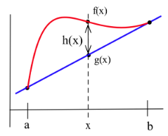
Fig. 6
The derivative of is =f^{\prime}(x)-g^{\prime}(x)") so we know that there is a number , between and , with . But
so we know that there is a number , between and , with . But =f^{\prime}(c)-g^{\prime}(c)") so
so =g^{\prime}(c)=\frac{f(b)-f(a)}{b-a}") .
.
Graphically, the Mean Value Theorem says that there is at least one point where the slope of the tangent line, , equals the slope of the line through the end points of the graph segment,
and . Fig. 7 shows the locations of the parallel tangent lines for several functions and intervals.
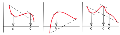
Fig. 7
The Mean Value Theorem also has a very natural interpretation if represents the position of an object at time ") represents the velocity of the object at the instant , and
represents the velocity of the object at the instant , and -\mathrm{f}(\mathrm{a})}{\mathrm{b}-\mathrm{a}}=\frac{\text
{ change in position }}{\text { change in time }}") represents the average (mean) velocity of the object during the time interval from time to time . The Mean Value Theorem says that there is a time , between
and , when the instantaneous velocity, , is equal to the average velocity for the entire trip,
represents the average (mean) velocity of the object during the time interval from time to time . The Mean Value Theorem says that there is a time , between
and , when the instantaneous velocity, , is equal to the average velocity for the entire trip, -\mathrm{f}(\mathrm{a})}{\mathrm{b}-\mathrm{a}}") . If your average velocity during a trip is
. If your average velocity during a trip is  miles per hour, then at some instant during the trip you were traveling exactly miles per hour.
Practice 2: For =5 x^{2}-4 x+3") on the interval
on the interval ![[1,3]](https://dev.saylor.org/filter/tex/pix.php/689e1b934020b6eb3917c155d94a9a0f.svg "[1,3]") , calculate
, calculate -f(a)}{b-a}") and find the value of so that
and find the value of so that =m") .
.
Some Consequences of the Mean Value Theorem
If the Mean Value Theorem was just an isolated result about the existence of a particular point , it would not be very important or useful. However, the Mean Value Theorem is the basis of several results about the behavior of functions over
entire intervals, and it is these consequences which give it an important place in calculus for both theoretical and applied uses.
The next two corollaries are just the first of many results which follow from the Mean Value Theorem.
We already know, from the Main Differentiation Theorem, that the derivative of a constant function. =k") is always , but can a nonconstant function have a derivative which is always ? The first corollary says no.
is always , but can a nonconstant function have a derivative which is always ? The first corollary says no.
Corollary 1: If =0") for all in an interval
for all in an interval  , then
 =\mathrm{K}") , a constant, for all in .
, a constant, for all in .
Proof: Assume for all in an interval , and pick any two points and ") in the interval. Then, by the Mean Value Theorem, there is a number
between and so that
in the interval. Then, by the Mean Value Theorem, there is a number
between and so that =\frac{\mathrm{f}(\mathrm{b})-\mathrm{f}(\mathrm{a})}{\mathrm{b}-\mathrm{a}}") . By our assumption, for all in
so we know that
. By our assumption, for all in
so we know that =\frac{\mathrm{f}(\mathrm{b})-\mathrm{f}(\mathrm{a})}{\mathrm{b}-\mathrm{a}}") and we can conclude that
and we can conclude that -\mathrm{f}(\mathrm{a})=0") and
and =\mathrm{f}(\mathrm{a})") .
But and were any two points in
.
But and were any two points in  , so the value of is the same for any two values of in , and is a constant function on the interval .
We already know that if two functions are parallel (differ by a constant), then their derivatives are equal, but can two nonparallel functions have the same derivative? The second corollary says no.
Corollary 2: If =g^{\prime}(x)") for all in an interval , then
for all in an interval , then -g(x)=K") , a constant, for all in , so the graphs of and are "parallel" on the interval .
, a constant, for all in , so the graphs of and are "parallel" on the interval .
Proof: This corollary involves two functions instead of just one, but we can imitate the proof of the Mean Value Theorem and introduce a new function =\mathrm{f}(\mathrm{x})-\mathrm{g}(\mathrm{x})") . The function
is differentiable, and
. The function
is differentiable, and =f^{\prime}(x)-g^{\prime}(x)=0") for all in , so, by Corollary
for all in , so, by Corollary ") is a constant function and
is a constant function and =\mathrm{f}(\mathrm{x})-\mathrm{g}(\mathrm{x})") for all
in the interval. Then
for all
in the interval. Then =\mathrm{g}(\mathrm{x})+\mathrm{K}") .
.
We will use Corollary 2 hundreds of times in Chapters 4 and 5 when we work with "integrals". Typically you will be given the derivative of a function, ") , and asked to find all functions which have that derivative. Corollary 2 tells
us that if we can find one function which has the derivative we want, then the only other functions which have the same derivative are
, and asked to find all functions which have that derivative. Corollary 2 tells
us that if we can find one function which has the derivative we want, then the only other functions which have the same derivative are +\mathrm{K}") : once you find one function with the right derivative, you
have essentially found all of them.
: once you find one function with the right derivative, you
have essentially found all of them.
Example 2: (a) Find all functions whose derivatives equal  .
.
(b) Find a function ") with
with =2 x") and
and =5") .
.
Solution: (a) We can recognize that if =\mathrm{x}^{2}") then
then =2 \mathrm{x}") so one function with the derivative we want is
so one function with the derivative we want is =x^{2}") . Corollary 2 guarantees that every function whose
derivative is
. Corollary 2 guarantees that every function whose
derivative is  has the form
 =\mathrm{f}(\mathrm{x})+\mathrm{K}=\mathrm{x}^{2}+\mathrm{K}") . The only functions with derivative have the form
. The only functions with derivative have the form  .
.
(b) Since , we know that must have the form =x^{2}+K") , but this is a whole "family" of functions (Fig. 8), and we want to find one member of the family . We know that so we want to find the member of the family
which goes through the point
, but this is a whole "family" of functions (Fig. 8), and we want to find one member of the family . We know that so we want to find the member of the family
which goes through the point ") . All we need to do is replace the with 5 and the with 3 in the formula
. All we need to do is replace the with 5 and the with 3 in the formula =\mathrm{x}^{2}+\mathrm{K}") , and then solve for the value of
, and then solve for the value of =(3)^{2}+\mathrm{K}") so
so  . The function we want is
 =x^{2}-4") .
.
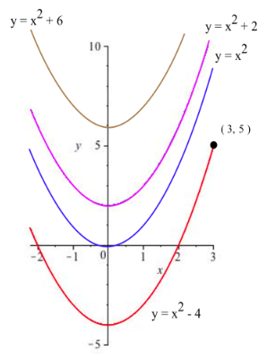
Fig. 8
Practice 3: Restate Corollary 2 as a statement about the positions and velocities of two cars.
Practice Answers
Practice 1: when  and
and  so
so  and
and  .
.
=0") when
when  , and so
  , and .
Practice 2: on . =4") and
and =36") so
so-\mathrm{f}(\mathrm{a})}{\mathrm{b}-\mathrm{a}}=\frac{36-4}{3-1}=16")
=10 \mathrm{x}-4") so
so =10 \mathrm{c}-4=16") if
if  and
and  .
.
The graph of and the location of are shown in Fig. 16.
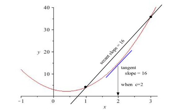
Fig. 16
Practice 3: If two cars have the same velocities during an interval of time (=\mathrm{g}^{\prime}(\mathrm{t})") for
for  in ) then the cars are always a constant distance
apart during that time interval.
in ) then the cars are always a constant distance
apart during that time interval.
(Note: The "same velocity" means same speed and same direction. If two cars are traveling at the same speed but in different directions, then the distance between them changes and is not constant)