The First Derivative and the Shape of a Function f(x)
| Site: | Saylor Academy |
| Course: | MA005: Calculus I |
| Book: | The First Derivative and the Shape of a Function f(x) |
| Printed by: | Guest user |
| Date: | Monday, October 21, 2024, 11:07 PM |
Description
Read this section to learn how the first derivative is used to determine the shape of functions. Work through practice problems 1-9.
The First Derivative and the Shape of a Function f
This section examines some of the interplay between the shape of the graph of  and the behavior of
  . If we have a graph of , we will see what we can conclude about the values of .
If we know values of , we will see what we can conclude about the graph of .
. If we have a graph of , we will see what we can conclude about the values of .
If we know values of , we will see what we can conclude about the graph of .
is increasing on ") if
if  implies
  < \mathrm{f}\left(\mathrm{x}_{2}\right)") .
. is decreasing on
 ") if
if  implies
  > f\left(x_{2}\right)") . is monotonic on
. is monotonic on ") if is increasing on
if is increasing on ") or if is decreasing on .
or if is decreasing on .Graphically, is increasing (decreasing) if, as we move from left to right along the graph of , the height of the graph increases (decreases).
These same ideas make sense if we consider ") to be the height (in feet) of a rocket at time
to be the height (in feet) of a rocket at time  seconds. We naturally say that the rocket is rising or that its height is increasing if the height
increases over a period of time, as increases.
seconds. We naturally say that the rocket is rising or that its height is increasing if the height
increases over a period of time, as increases.
Example 1: List the intervals on which the function given in Fig. 1 is increasing or decreasing.

Fig. 1
Solution: is increasing on the intervals ![[0,1],[2,3]](https://dev.saylor.org/filter/tex/pix.php/402240a0c1f22e535db19caae6c4dd19.svg "[0,1],[2,3]") and
and ![[4,6]](https://dev.saylor.org/filter/tex/pix.php/06ed86e533acc38ab36f76bbef4dd412.svg "[4,6]") . is decreasing on
. is decreasing on ![[1,2]](https://dev.saylor.org/filter/tex/pix.php/f79408e5ca998cd53faf44af31e6eb45.svg "[1,2]") and
and ![[6,8]](https://dev.saylor.org/filter/tex/pix.php/6b005fc2af378ca9d250fffeccfce487.svg "[6,8]") . On the interval
. On the interval ![[3,4]](https://dev.saylor.org/filter/tex/pix.php/b814fa889082069ffb727ee1623c0944.svg "[3,4]") the function is not increasing or decreasing, it is constant. It is also valid to
say that is increasing on the intervals
the function is not increasing or decreasing, it is constant. It is also valid to
say that is increasing on the intervals ![[0.3,0.8]](https://dev.saylor.org/filter/tex/pix.php/a17f8dc40b69bd89797962059d5a97f7.svg "[0.3,0.8]") and
and ") as well as many others, but we usually talk about the longest intervals on which is monotonic.
as well as many others, but we usually talk about the longest intervals on which is monotonic.
Practice 1: List the intervals on which the function given in Fig. 2 is increasing or decreasing.
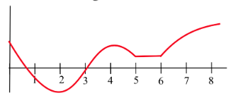
Fig. 2
If we have an accurate graph of a function, then it is relatively easy to determine where is monotonic, but if the function is defined by an equation, then a little more work is required. The next two theorems relate the values of the derivative
of to the monotonicity of . The first theorem says that if we know where is monotonic, then we also know something about the values of  . The second theorem says that if we know about the values of
then we can draw conclusions about where is monotonic.
. The second theorem says that if we know about the values of
then we can draw conclusions about where is monotonic.
First Shape Theorem
For a function which is differentiable on an interval ;
(i) if is increasing on , then  \geq 0") for all
for all  in
in
(ii) if is decreasing on ") , then
, then  \leq 0") for all
for all  in
in
(iii) if is constant on , then =0") for all in .
for all in .
Proof: Most people find a picture such as Fig. 3 to be a convincing justification of this theorem: if the graph of increases near a point )") , then the tangent line is also increasing, and the slope of the tangent line is positive (or
perhaps zero at a few places). A more precise proof, however, requires that we use the definitions of the derivative of and of "increasing".
, then the tangent line is also increasing, and the slope of the tangent line is positive (or
perhaps zero at a few places). A more precise proof, however, requires that we use the definitions of the derivative of and of "increasing".
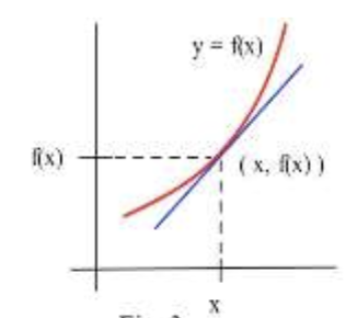
Fig. 3
(i) Assume that is increasing on . We know that is differentiable, so if is any number in the interval then =\lim _{h \rightarrow 0} \frac{f(x+h)-f(x)}{h}") , and
this limit exists and is a finite value.
, and
this limit exists and is a finite value.
If  is any small enough positive number so that
  is also in the interval , then
  and
and  < f(x+h)") . We know that the numerator,
. We know that the numerator, -f(x)") , and the denominator, , are both positive
so the limiting value,
, and the denominator, , are both positive
so the limiting value, ") , must be positive or zero: .
, must be positive or zero: .
(ii) Assume that is decreasing on : The proof of this part is very similar to part (i). If , then  > f(x+h)") since is decreasing on . Then the numerator of the limit, , will be negative
and the denominator,
since is decreasing on . Then the numerator of the limit, , will be negative
and the denominator,  , will still be positive, so the limiting value,
 ") , must be negative or zero:
, must be negative or zero:  \leq 0") .
.
(iii) The derivative of a constant is zero, so if is constant on then =0") for all in .
for all in .
The previous theorem is easy to understand, but you need to pay attention to exactly what it says and what it does not say. It is possible for a differentiable function which is increasing on an interval to have horizontal tangent lines at some places in the interval (Fig 4).
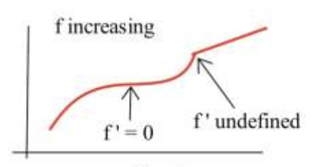
Fig. 4
It is also possible for a continuous function which is increasing on an interval to have an undefined derivative at some places in the interval (Fig. 4).
Finally, it is possible for a function which is increasing on an interval to fail to be continuous at some places in the interval (Fig. 5).
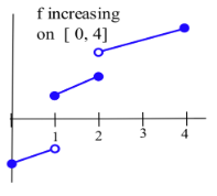
Fig. 5
The First Shape Theorem has a natural interpretation in terms of the height and upward velocity ") of a helicopter at time
of a helicopter at time  . If the height of the helicopter is increasing (
is increasing ), then the helicopter has a positive or zero upward velocity:
. If the height of the helicopter is increasing (
is increasing ), then the helicopter has a positive or zero upward velocity:  \geq 0") . If the height of the helicopter is not changing, then its upward velocity is
. If the height of the helicopter is not changing, then its upward velocity is =0") .
.
Example 2: Fig. 6 shows the height of a helicopter during a period of time. Sketch the graph of the upward velocity of the helicopter,  .
.
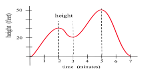
Fig. 6
Solution: The graph of =\mathrm{dh} / \mathrm{dt}") is shown in Fig.7. Notice that the has a local maximum when
is shown in Fig.7. Notice that the has a local maximum when  and
and  , and
, and =0") and
and =0") .
Similarly, has a local minimum when
.
Similarly, has a local minimum when  , and
, and =0") . When is increasing,
. When is increasing,  is positive. When is decreasing,
  is negative.

Fig. 7
Practice 2: Fig. 8 shows the population of rabbits on an island during 6 years. Sketch the graph of the rate of population change,  , during those years.

Fig. 8
Example 3: The graph of is shown in Fig. 9. Sketch the graph of .
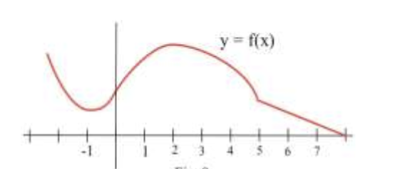
Fig. 9
Solution: It is a good idea to look first for the points where or where is not differentiable, the critical points of . These locations are usually easy to spot, and they naturally break the problem into several smaller
pieces. The only numbers at which are  and
and  , so the only places the graph of will cross the -axis are at and , and we can plot the point
 ") and
and ") on the graph
of
on the graph
of  . The only place that is not differentiable is at the "corner" above
  , so the graph of will not have a point for . The rest of the graph of is relatively easy:
if  then
then ") is decreasing so is negative,
is decreasing so is negative,
if  then is increasing so is positive,
if  then is decreasing so is negative, and
if  then is decreasing so is negative.
The graph of  is shown in Fig. 10.
 ") is continuous at
is continuous at  , but is not differentiable at , as is indicated by the "hole" in the graph.
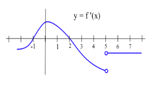
Fig. 10
Practice 3: The graph of is shown in Fig. 11. Sketch the graph of . (The graph of has a "corner" at .)
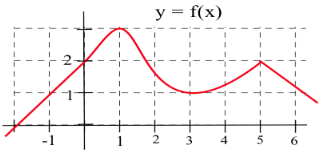
Fig. 11
The next theorem is almost the converse of the First Shape Theorem and explains the relationship between the values of the derivative and the graph of a function from a different perspective. It says that if we know something about the values of ,
then we can draw some conclusions about the shape of the graph of .
Second Shape Theorem
For a function which is differentiable on an interval I;
(i) if  > 0") for all in the interval
for all in the interval  , then is increasing on ,
(ii) if 
< 0") for all in the interval , then is decreasing on ,
for all in the interval , then is decreasing on ,
(iii) if for all in the interval , then is
constant on .
Proof: This theorem follows directly from the Mean Value Theorem, and part (c) is just a restatement of the First Corollary of the Mean Value Theorem.
(a) Assume that for all in and pick any points a and  in with
  . Then, by the Mean Value Theorem, there is a point
  between
  and
and  so that
 -f(a)}{b-a}=f^{\prime}(c) > 0") , and we can conclude that
, and we can conclude that -\mathrm{f}(\mathrm{a}) > 0") and
and  > \mathrm{f}(\mathrm{a})") . Since
implies that
. Since
implies that  < \mathrm{f}(\mathrm{b})") , we know that is increasing on
, we know that is increasing on  .
.
(b) Assume that  < 0") for all in and pick any points and in with . Then there is a point between and
so that
for all in and pick any points and in with . Then there is a point between and
so that -f(a)}{b-a}=f^{\prime}(c) < 0") , and we can conclude that
, and we can conclude that -\mathrm{f}(\mathrm{a})=(\mathrm{b}-\mathrm{a}) \mathrm{f}^{\prime}(\mathrm{c}) < 0") so
so  < \mathrm{f}(\mathrm{a})") .
Since implies that
.
Since implies that  > \mathrm{f}(\mathrm{b})") , we know is decreasing on .
, we know is decreasing on .
Practice 4: Rewrite the Second Shape Theorem as a statement about the height and upward velocity of a helicopter at time seconds.
The value of the function at a number tells us the height of the graph of above or below the point on the -axis. The value of at a number tells us whether the graph of is increasing or decreasing (or neither)
as the graph passes through the point on the graph of . If is positive, it is possible for to be positive, negative, zero or undefined: the value of has absolutely
nothing to do with the value of . Fig. 12 illustrates some of the combinations of values for and .

Fig. 12
Practice 5: Graph a continuous function which satisfies the conditions on and given below
 & 1 & -1 & -2 & -1 & 0 & 2 \\\hline \mathrm{f}^{\prime}(\mathrm{x}) & -1 & 0 & 1
& 2 & -1 & 1\end{array}")
The Second Shape Theorem is particularly useful if we need to graph a function which is defined by an equation. Between any two consecutive critical numbers of , the graph of is monotonic (why?). If we can find
all of the critical numbers of , then the domain of will be naturally broken into a number of pieces on which will be monotonic.
Example 4: Use information about the values of to help graph =\mathrm{x}^{3}-6 \mathrm{x}^{2}+9 \mathrm{x}+1") .
.
Solution: =3 \mathrm{x}^{2}-12 \mathrm{x}+9=3(\mathrm{x}-1)(\mathrm{x}-3)") so only when
so only when  or
or  . is a polynomial so it is always
defined. The only critical numbers for are and
. is a polynomial so it is always
defined. The only critical numbers for are and  , and they divide the real number line into three pieces on which is monotonic:
 ,(1,3)") and
and ") .
.
If  , then
 =3") (negative number)(negative number)
(negative number)(negative number)  so is increasing.
If  , then (positive number)(negative number)
  so is decreasing.
If  , then (positive number)(positive number) so is increasing.
Even though we don't know the value of anywhere yet, we do know a lot about the shape of the graph of : as we move from left to right along the -axis, the graph of increases until  , then the graph decreases until
, and then the graph increases again (Fig. 13) The graph of makes "turns" when and .
, then the graph decreases until
, and then the graph increases again (Fig. 13) The graph of makes "turns" when and .
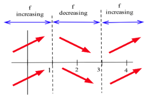
Fig. 13
To plot the graph of , we still need to evaluate at a few values of , but only at a very few values. =5") , and
, and ") is a local maximum of .
is a local maximum of . =1") , and
, and ") is a local minimum of . The graph
of is shown in Fig. 14.
is a local minimum of . The graph
of is shown in Fig. 14.

Fig. 14
Practice 6: Use information about the values of to help graph =\mathrm{x}^{3}-3 \mathrm{x}^{2}-24 \mathrm{x}+5") .
.
Example 5: Use the graph of in Fig. 15 to sketch the shape of the graph of . Why isn't the graph of enough to completely determine the graph of ?
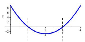
Fig. 15
Solution: Several functions which have the derivative we want are given in Fig. 16 , and each of them is a correct answer. By the Second Corollary to the Mean Value Theorem, we know there is a whole family of parallel functions which have the derivative
we want, and each of these functions is a correct answer. If we had additional information about the function such as a point it went through, then only one member of the family would satisfy the extra condition and that function would be the only
correct answer.
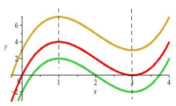
Fig. 16
Practice 7: Use the graph of  in Fig. 17 to sketch the shape of a graph of
  .
.
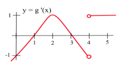
Fig. 17
Practice 8: A weather balloon is released from the ground and sends back its upward velocity measurements (Fig. 18). Sketch a graph of the height of the balloon. When was the balloon highest?

Fig. 18
Source: Dale Hoffman, https://s3.amazonaws.com/saylordotorg-resources/wwwresources/site/wp-content/uploads/2012/12/MA005-4.3-First-Derivative.pdf This work is licensed under a Creative Commons Attribution 3.0 License.
Using the Derivative to Test for Extremes
The first derivative of a function tells about the general shape of the function, and we can use that shape information to determine if an extreme point is a maximum or minimum or neither.
First Derivative Test for Local Extremes
Let be a continuous function with =0") or
or ") is undefined.
is undefined.
(i) If (left of ) and (right of ) , then )") is a local maximum (Fig. 19a)
is a local maximum (Fig. 19a)
(ii) If (left of )  and (right of )
  , then is a local minimum (Fig. 19b)
(iii) If (left of ) and (right of ) , then is not a local extreme (Fig. 19c)
(iv) If (left of ) and (right of ) , then is not a local extreme (Fig. 19d)
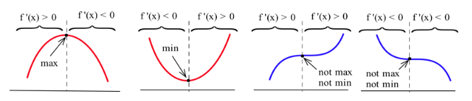
Fig. 19
Practice 9: Find all extremes of =3 x^{2}-12 x+7") and use the First Derivative Test to determine if they are maximums, minimums or neither.
and use the First Derivative Test to determine if they are maximums, minimums or neither.
A variant of the First Derivative Test can also be used to determine whether an endpoint gives a maximum or minimum for a function.
Practice Answers
Practice 1: is increasing on ![[2,4]](https://dev.saylor.org/filter/tex/pix.php/a157b852663a42e907fc1ae4884ff3e4.svg "[2,4]") and . is decreasing on
and . is decreasing on ![[0,2]](https://dev.saylor.org/filter/tex/pix.php/70fd3f388413505934da60b43afc4088.svg "[0,2]") and
and ![[4,5]](https://dev.saylor.org/filter/tex/pix.php/30eeb203d66f0c29522e851b605d8a9e.svg "[4,5]") ,
, is constant on
 ![[5,6]](https://dev.saylor.org/filter/tex/pix.php/9e2c1d72e747415c20b12330213b66e7.svg "[5,6]") .
.
Practice 2: The graph in Fig. 33 shows the rate of population change, .

Fig. 33
Practice 3: The graph of is shown in Fig. 34. Notice how the graph of is  where has a maximum and minimum.
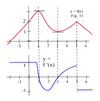
Fig. 34
Practice 4: The Second Shape Theorem for helicopters:
(i) If the upward velocity  is positive during time interval then the height is increasing during time interval .
(ii) If the upward velocity
is negative during time interval then the height is decreasing during time interval .
(iii) If the upward velocity is zero during time interval then the height is constant during
time interval .
Practice 5: A graph satisfying the conditions in the table is shown in Fig. 35.
 & 1 & -1 & -2 & -1 & 0 & 2 \\\hline \mathrm{f}^{\prime}(\mathrm{x}) & -1 & 0 & 1
& 2 & -1 & 1\end{array}")
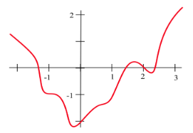
Fig. 35
Practice 6: .
=3 \mathrm{x}^{2}-6 \mathrm{x}-24=3(\mathrm{x}-4)(\mathrm{x}+2)") .
.
if  .
.
If 
then =3(x-4)(x+2)=3") (negative) (negative) so is increasing.
(negative) (negative) so is increasing.
If 
then =3(\mathrm{x}-4)(\mathrm{x}+2)=3") (negative)(positive) so is decreasing.
(negative)(positive) so is decreasing.
If 
then (positive) (positive) so is increasing
has a relative maximum at  and a relative minimum at
  .
.
The graph of is shown in Fig. 36.
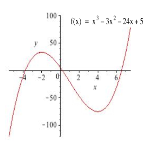
Fig. 36
Practice 7: Fig. 37 shows several possible graphs for . Each of the graphs has the correct shape to give the graph of . Notice that the graphs of are "parallel," differ by a constant.

Fig. 37
Practice 8: Fig. 38 shows the height graph for the balloon. The balloon was highest at  and had a local minimum at
  .
.
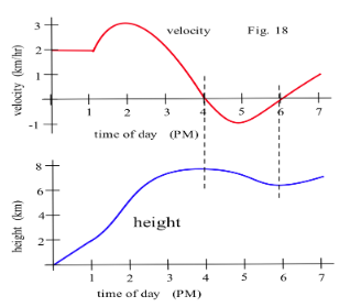
Fig. 38
Practice 9: so =6 x-12") .
.
if .
If  , then
  < 0") and is decreasing.
and is decreasing.
If  , then
  > 0") and
is increasing.
and
is increasing.
From this we can conclude that has a minimum when  and has a shape similar to Fig. 19(b).
We could also notice that the graph of the quadratic is an upward opening parabola. The graph of is shown in Fig. 39.

Fig. 39