Derivative Patterns

If we apply the Product Rule to the product of a function with itself, a familiar pattern emerges. 

$\begin{align*}\begin{aligned}&D\left(f^{2}\right)=D(f \cdot f)=f \cdot D(f)+f \cdot D(f)=2 f \cdot D(f) \\&D\left(f^{3}\right)=D\left(f^{2} \cdot f\right)=f^{2} \cdot \mathbf{D}(f)+f \cdot D\left(f^{2}\right)=f^{2} \cdot \mathbf{D}(f)+f\{2 f \cdot D(f)\}=f^{2} \cdot \mathbf{D}(f)+2 f^{2} \cdot \mathbf{D}(f)=3 f^{2} \cdot \mathbf{D}(f) \\&D\left(f^{4}\right)=D\left(f^{3} \cdot f\right)=f^{3} \cdot \mathbf{D}(f)+f \cdot D\left(f^{3}\right)=f^{3} \cdot \mathbf{D}(f)+f\left\{3 f^{2} \cdot \mathbf{D}(f)\right\}=f^{3} \cdot \mathbf{D}(f)+3 f^{3} \cdot \mathbf{D}(f)=4 f^{3} \cdot \mathbf{D}(\mathbf{f})\end{aligned}\end{align*}$

Practice 1: What is the pattern here? What do you think the results will be for $\mathbf{D}\left(\mathrm{f}^{5}\right)$ and $\mathrm{D}\left(\mathrm{f}^{13}\right)$?

We could keep differentiating higher and higher powers of $f(x)$ by writing them as products of lower powers of $f(x)$ and using the Product Rule, but the Power Rule For Functions guarantees that the pattern we just saw for the small integer powers also works for all constant powers of functions. 

Power Rule For Functions: If $\mathrm{n}$ is any constant,

then $\begin{align*}\quad \mathbf{D}\left(f^{n}(x)\right)=n f^{n-1}(x) \cdot \mathbf{D}(\mathbf{f}(x))\end{align*}$

The Power Rule for Functions is a special case of a more general theorem, the Chain Rule, which we will examine in Section 2.4. The Power Rule For Functions will be proved after the Chain Rule.

Example 1: Use the Power Rule for Functions to find

(a) $\mathbf{D}\left(\left(\mathrm{x}^{3}-5\right)^{2}\right)$

(b) $\frac{\mathbf{d}}{\mathrm{dx}}\left(\sqrt{2 \mathrm{x}+3 \mathrm{x}^{5}}\right)$

(c) $\mathbf{D}\left(\sin ^{2}(\mathrm{x})\right)=\mathbf{D}\left((\sin (\mathrm{x}))^{2}\right)$.

Solution: (a) To match the pattern of the Power Rule for $\mathbf{D}\left(\left(x^{3}-5\right)^{2}\right)$, let $f(x)=x^{3}-5$ and $n=2$.

Then $\mathbf{D}\left(\left(x^{3}-5\right)^{2}\right)=\mathbf{D}\left(f^{n}(x)\right)=n f^{n-1}(x) \cdot \mathbf{D}(f(x))$

$\begin{align*}=2\left(x^{3}-5\right)^{1} D\left(x^{3}-5\right)=2\left(x^{3}-5\right)\left(3 x^{2}\right)=6 x^{2}\left(x^{3}-5\right)\end{align*}$

(b) To match the pattern for $\frac{\mathbf{d}}{\mathrm{dx}}\left(\sqrt{2 \mathrm{x}+3 \mathrm{x}^{5}}\right)=\frac{\mathbf{d}}{\mathbf{d x}}\left(\left(2 \mathrm{x}+3 \mathrm{x}^{5}\right)^{1 / 2}\right)$, we can let $\mathrm{f}(\mathrm{x})=2 \mathrm{x}+3 \mathrm{x}^{5}$ and take $\mathrm{n}=1 / 2$. Then

$\begin{align*}\begin{aligned}\frac{\mathbf{d}}{\mathbf{d x}}\left(\left(2 \mathrm{x}+3 \mathrm{x}^{5}\right)^{1 / 2}\right) &=\frac{\mathbf{d}}{d \mathrm{x}}\left(\mathrm{f}^{\mathrm{n}}(\mathrm{x})\right)=\mathrm{n} \mathrm{f}^{\mathrm{n}-1}(\mathrm{x}) \cdot \frac{\mathbf{d}}{\mathrm{dx}}(\mathrm{f}(\mathrm{x}))=\frac{1}{2}\left(2 \mathrm{x}+3 \mathrm{x}^{5}\right)^{-1 / 2} \frac{\mathbf{d}}{\mathrm{dx}}\left(2 \mathrm{x}+3 \mathrm{x}^{5}\right) \\&=\frac{1}{2}\left(2 \mathrm{x}+3 \mathrm{x}^{5}\right)^{-1 / 2}\left(2+15 \mathrm{x}^{4}\right)=\frac{2+15 \mathrm{x}^{4}}{2 \sqrt{2 \mathrm{x}+3 \mathrm{x}^{5}}}\end{aligned}\end{align*}$

(c) To match the pattern for $\mathbf{D}\left(\sin ^{2}(x)\right)$, Let $f(x)=\sin (x)$ and $n=2$. Then

$\begin{align*}\mathbf{D}\left(\sin ^{2}(\mathrm{x})\right) \quad=\mathbf{D}\left(\mathrm{f}^{\mathrm{n}}(\mathrm{x})\right) \quad=\mathrm{n} \mathrm{f}^{\mathrm{n}-1}(\mathrm{x}) \cdot \mathbf{D}(\mathrm{f}(\mathrm{x}))=2 \sin ^{1}(\mathrm{x}) \mathbf{D}(\sin (\mathrm{x}))=2 \sin (\mathbf{x}) \cos (\mathbf{x})\end{align*}$

Practice 2: Use the Power Rule for Functions to find

(a) $\frac{\mathbf{d}}{\mathbf{d x}}\left(\left(2 \mathrm{x}^{5}-\pi\right)^{2}\right)$,

(b) $\mathbf{D}\left(\sqrt{x+7 x^{2}}\right)$

(c) $\mathbf{D}\left(\cos ^{4}(x)\right)=\mathbf{D}\left((\cos (x))^{4}\right)$.

Example 2: Use calculus to show that the line tangent to the circle $x^{2}+y^{2}=25$ at the point $(3,4)$ has slope $-3 / 4$.

Solution: The top half of the circle is the graph of $y=f(x)=\sqrt{25-x^{2}}$ so $f^{\prime}(x)=D\left(\left(25-x^{2}\right)^{1 / 2}\right)$

$\begin{align*}=\frac{1}{2}\left(25-\mathrm{x}^{2}\right)^{-1 / 2} \mathrm{D}\left(25-\mathrm{x}^{2}\right)=\frac{-\mathrm{x}}{\sqrt{25-\mathrm{x}^{2}}} \end{align*}$ and $\quad\mathrm{f}^{\prime}(3)=\frac{-3}{\sqrt{25-3^{2}}}=\frac{-3}{4}$

As a check, you can verify that the slope of the radial line through the center of the circle $(0,0)$ and the point $(3,4)$ has slope $4 / 3$ and is perpendicular to the tangent line which has a slope of $-3 / 4$.

We have some general rules which apply to any elementary combination of differentiable functions, but in order to use the rules we still need to know the derivatives of each of the particular functions. Here we will add to the list of functions whose derivatives we know.

Derivatives of the Trigonometric Functions 

We know the derivatives of the sine and cosine functions, and each of the other four trigonometric functions is just a ratio involving sines or cosines. Using the Quotient Rule, we can differentiate the rest of the trigonometric functions. 

$\begin{array}{lll} \text { Theorem: } & \mathbf{D}(\tan (x)) \quad=\quad \sec ^{2}(x) & D(\sec (x))=\quad \sec (x) \tan (x) \\ & D(\cot (x)) \quad=-\csc ^{2}(x) & D(\csc (x))=-\csc (x) \cot (x) \end{array}$

Proof: From trigonometry we know $\tan (x)=\frac{\sin (x)}{\cos (x)}, \cot (x)=\frac{\cos (x)}{\sin (x)}, \sec (x)=\frac{1}{\cos (x)}$, and $\csc (x)=\frac{1}{\sin (x)}$ and we know $\mathbf{D}(\sin (x))=\cos (x)$ and $D(\cos (x))=-\sin (x) .$ Using the Quotient Rule,

$\begin{align*} \begin{aligned} &\mathbf{D}(\tan (\mathrm{x}))=\mathbf{D}\left(\frac{\sin (\mathrm{x})}{\cos (\mathrm{x})}\right)=\frac{\cos (\mathrm{x}) \cdot \mathrm{D}(\sin (\mathrm{x}))-\sin (\mathrm{x}) \cdot \mathrm{D}(\cos (\mathrm{x}))}{(\cos (\mathrm{x}))^{2}} \\ &=\frac{\cos (\mathrm{x}) \cos (\mathbf{x})-\sin (\mathrm{x})\{-\sin (\mathbf{x})\}}{\cos ^{2}(\mathrm{x})}=\frac{\cos ^{2}(\mathrm{x})+\sin ^{2}(\mathrm{x})}{\cos ^{2}(\mathrm{x})}=\frac{1}{\cos ^{2}(\mathrm{x})}=\sec ^{2}(\mathbf{x}) \\ &=\frac{\cos (\mathrm{x})(\mathbf{0})-1\{-\sin (\mathbf{x})\}}{\cos ^{2}(\mathrm{x})}=\frac{\sin (\mathrm{x})}{\cos ^{2}(\mathrm{x})}=\frac{\sin (\mathrm{x})}{\cos (\mathrm{x})} \frac{1}{\cos (\mathrm{x})}=\tan (\mathbf{x}) \cdot \sec (\mathrm{x}) \end{aligned} \end{align*}$

Instead of the Quotient Rule, we could have used the Power Rule to calculate $\mathbf{D}(\sec (x))=\mathbf{D}\left((\cos (\mathrm{x}))^{-1}\right)$.

Practice 3: Use the Quotient Rule on $f(x)=\cot (x)=\frac{\cos (x)}{\sin (x)}$ to prove that f $^{\prime}(x)=-\csc ^{2}(x)$.

Practice 4: Prove that $\mathbf{D}(\csc (x))=-\csc (x) \cdot \cot (x)$. The justification of this result is very similar to the justification for $\mathbf{D}(\sec (\mathrm{x}))$

Practice 5: Find (a) $\mathbf{D}\left(\mathrm{x}^{5} \cdot \tan (\mathrm{x})\right)$, (b) $\frac{\mathbf{d}}{\mathrm{dt}}\left(\frac{\sec (\mathrm{t})}{\mathrm{t}}\right)$ and (c) $\mathrm{D}(\sqrt{\cot (\mathrm{x})-\mathrm{x}})$.

Derivative of $e^x$ 

We can use graphs of exponential functions to estimate the slopes of their tangent lines or we can numerically approximate the slopes.

Example 3: Estimate the derivative of $\mathrm{f}(\mathrm{x})=2^{\mathrm{X}}$ at the point $\left(0,2^{0}\right)=(0,1)$ by approximating the slope of the line tangent to $\mathrm{f}(\mathrm{x})=2^{\mathrm{X}}$ at that point

Solution: We can get estimates from the graph of $\mathrm{f}(\mathrm{x})=2^{\mathrm{X}}$ by carefully graphing $\mathrm{f}(\mathrm{x})=2^{\mathrm{X}}$ for small values of $\mathrm{x}$, sketching secant lines, and then measuring the slopes of the secant lines (Fig. 1).

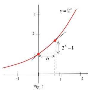
We can also find the slope numerically by using the definition of the derivative,

$\mathrm{f}^{\prime}(0) \equiv \lim\limits_{h \rightarrow 0} \frac{f(0+h)-f(0)}{h}=\lim\limits_{h \rightarrow 0} \frac{2^{0+h}-2^{0}}{h}=\lim\limits_{h \rightarrow 0} \frac{2^{h}-1}{h}$, and evaluating $\frac{2^{\mathrm{h}}-1}{\mathrm{~h}}$ for some very small values of $\mathrm{h}$.

From the table we can see that $f ' (0) ≈ .693$.

Practice 6: Fill in the table for $\frac{3^{\mathrm{h}}-1}{\mathrm{~h}}$, and show that the slope of the line tangent to $\mathrm{g}(\mathrm{x})=3^{\mathrm{x}}$ at $(0,1)$ is approximately $1.099$. (Fig. 2)

At $(0,1)$, the slope of the tangent to $y=2^{x}$ is less than 1, and the slope of the tangent to $\mathrm{y}=3^{\mathrm{x}}$ is slightly greater than 1. (Fig. 3) There is a number, denoted $\mathbf{e}$, between 2 and 3 so that the slope of the tangent to $\mathrm{y}=\mathrm{e}^{\mathrm{x}}$ is exactly 1: $\lim\limits_{h \rightarrow 0} \frac{e^{h}-1}{h}=1 .$ The number $\mathrm{e} \approx 2.71828182845904$.

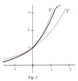
$e$ is irrational and is very important and common in calculus and applications.

Once we grant that $\lim _{h \rightarrow 0} \frac{e^{h}-1}{h}=1$, it is relatively straightforward to calculate $\mathbf{D}\left(\mathrm{e}^{\mathrm{x}}\right)$.

Theorem: $D(e^X) = e^X$

Proof:

$\begin{align*} \begin{aligned} \mathbf{D}\left(\mathrm{e}^{\mathrm{x}}\right) & \equiv \lim\limits_{h \rightarrow 0} \frac{e^{x+h}-e^{x}}{h}=\lim\limits_{h \rightarrow 0} \frac{e^{x} \cdot e^{h}-e^{x}}{h} \\ &=\lim\limits_{h \rightarrow 0}\left(e^{x}\right) \cdot\left(\frac{e^{h}-1}{h}\right) \\ &=\lim\limits_{h \rightarrow 0}\left(e^{x}\right) \cdot \lim\limits_{h \rightarrow 0}\left(\frac{e^{h}-1}{h}\right)=\left(\mathrm{e}^{\mathrm{x}}\right)(1)=\mathbf{e}^{\mathbf{x}} . \end{aligned} \end{align*}$

The function $f(x)=e^{x}$ is its own derivative: $f^{\prime}(x)=f(x)$. The height of $f(x)=e^{x}$ at any point and the slope of the tangent to $\mathrm{f}(\mathrm{x})=\mathrm{e}^{\mathrm{x}}$ at that point are the same: as the graph gets higher, its slope gets steeper.

Example 4: Find (a) $\frac{\mathbf{d}}{d t}\left(t \cdot e^{t}\right)$, (b) $D\left(e^{x} / \sin (x)\right)$ and (c) $D\left(e^{5 x}\right)=D\left(\left(e^{x}\right)^{5}\right)$

Solution: (a) Using the Product Rule with $\mathrm{f}(\mathrm{t})=\mathrm{t}$ and $\mathrm{g}(\mathrm{t})=\mathrm{e}^{\mathrm{t}}$,

$\begin{align*} \frac{\mathbf{d}}{\mathbf{d t}}\left(t \cdot e^{t}\right)=t \cdot \mathbf{D}\left(\mathrm{e}^{\mathrm{t}}\right)+\mathrm{e}^{\mathrm{t}} \cdot \mathbf{D}(\mathrm{t})=\mathrm{t} \cdot \mathbf{e}^{\mathbf{t}}+\mathrm{e}^{\mathrm{t}} \cdot(\mathbf{1})=\mathrm{t} \cdot \mathrm{e}^{\mathrm{t}}+\mathrm{e}^{\mathrm{t}}=(\mathrm{t}+1) \mathrm{e}^{\mathrm{t}} \end{align*}$

(b) Using the Quotient Rule with $\mathrm{f}(\mathrm{x})=\mathrm{e}^{\mathrm{x}}$ and $\mathrm{g}(\mathrm{x})=\sin (\mathrm{x})$,

$\begin{align*} \mathbf{D}\left(\frac{\mathrm{e}^{\mathrm{x}}}{\sin (\mathrm{x})}\right)=\frac{\sin (\mathrm{x}) \mathbf{D}\left(\mathrm{e}^{\mathrm{x}}\right)-\mathrm{e}^{\mathrm{x}} \mathbf{D}(\sin (\mathrm{x}))}{\sin ^{2}(\mathrm{x})}=\frac{\sin (\mathrm{x}) \mathrm{e}^{\mathbf{x}}-\mathrm{e}^{\mathrm{x}} \cos (\mathbf{x})}{\sin ^{2}(\mathrm{x})} \end{align*}$

(c) Using the Power Rule for Functions with $\mathrm{f}(\mathrm{x})=\mathrm{e}^{\mathrm{x}}$ and $\mathrm{n}=5$,

$\begin{align*} D\left(\left(e^{x}\right)^{5}\right)=5\left(e^{x}\right)^{4} \cdot D\left(e^{x}\right)=5\left(e^{x}\right)^{4} \cdot e^{x}=5 e^{4 x} e^{x}=5 e^{5 x} \end{align*}$

Practice 7: Find (a) $\mathrm{D}\left(\mathrm{x}^{3} \mathrm{e}^{\mathrm{x}}\right)$ and (b) $\mathrm{D}\left(\left(\mathrm{e}^{\mathrm{x}}\right)^{3}\right)$.

The derivative of a function $\mathrm{f}$ is a new function $\mathbf{f}^{\prime}$, and we can calculate the derivative of this new function to get the derivative of the derivative of $f$, denoted by $f^{\prime \prime}$ and called the second derivative of $f$. For example, if $f(x)=x^{5}$ then $f^{\prime}(x)=5 x^{4}$ and $f^{\prime \prime}(x)=\left(f^{\prime}(x)\right)^{\prime}=\left(5 x^{4}\right)^{\prime}=20 x^{3}$.

Definitions: The first derivative of $\mathrm{f}$ is $\mathrm{f}^{\prime}(\mathrm{x})$, the rate of change of $\mathrm{f}$.

The second derivative of $f$ is $f^{\prime \prime}(x)=\left(f^{\prime}(x)\right)^{\prime}$, the rate of change of $f^{\prime}$. The third derivative of $f$ is $f^{\prime \prime \prime}(x)=\left(f^{\prime \prime}(x)\right)^{\prime}$, the rate of change of $f$ ".

For $y=f(x), f^{\prime}(x)=\frac{d y}{d x}, f^{\prime \prime}(x)=\frac{d}{d x}\left(\frac{d y}{d x}\right)=\frac{d^{2} y}{d x^{2}}, f^{\prime \prime \prime}(x)=\frac{d}{d x}\left(\frac{d^{2} y}{d x^{2}}\right)=\frac{d^{3} y}{d x^{3}}$, and so on.

Practice 8: Find $\mathrm{f}^{\prime}, \mathrm{f} "$, and $\mathrm{f}^{\prime \prime \prime}$ for $\mathrm{f}(\mathrm{x})=3 \mathrm{x}^{7}, \mathrm{f}(\mathrm{x})=\sin (\mathrm{x})$, and $\mathrm{f}(\mathrm{x})=\mathrm{x} \cos (\mathrm{x})$

If $\mathrm{f}(\mathrm{x})$ represents the position of a particle at time $\mathrm{x}$, then $\mathrm{v}(\mathrm{x})=\mathrm{f}^{\prime}(\mathrm{x})$ will represent the velocity (rate of change of the position) of the particle and $\mathrm{a}(\mathrm{x})=\mathrm{v}^{\prime}(\mathrm{x})=\mathrm{f}^{\prime \prime}(\mathrm{x})$ will represent the acceleration (the rate of change of the velocity) of the particle.

Example 5: The height (feet) of a particle at time $\mathrm{t}$ seconds is $\mathrm{t}^{3}-4 \mathrm{t}^{2}+8 \mathrm{t}$. Find the height, velocity and acceleration of the particle when $\mathrm{t}=0,1$, and $2$ seconds.

Solution: $f(t)=t^{3}-4 t^{2}+8 t$ so $f(0)=0$ feet, $f(1)=5$ feet, and $f(2)=8$ feet

The velocity is $v(t)=f^{\prime}(t)=3 t^{2}-8 t+8$ so $v(0)=8 \mathrm{ft} / \mathrm{s}, v(1)=3 \mathrm{ft} / \mathrm{s}$, and $\mathrm{v}(2)=4 \mathrm{ft} / \mathrm{s}$. At each of these times the velocity is positive and the particle is moving upward, increasing in height.

The acceleration is $a(t)=6 t-8$ so $a(0)=-8 \mathrm{ft} / \mathrm{s}^{2}, a(1)=-2 \mathrm{ft} / \mathrm{s}^{2}$ and $\mathrm{a}(2)=4 \mathrm{ft} / \mathrm{s}^{2}$.

We will examine the geometric meaning of the second derivative later.

In Section 1.2 we saw that the "holey" function $\mathrm{h}(\mathrm{x})= \begin{cases}2 & \text { if } \mathrm{x} \text { is a rational number } \\ 1 & \text { if } \mathrm{x} \text { is an irrational number }\end{cases}$

is discontinuous at every value of $x$, so at every $x$  $h(x)$ is not differentiable. We can create graphs of continuous functions that are not differentiable at several places just by putting corners at those places, but how many corners can a continuous function have? How badly can a continuous function fail to be differentiable? 

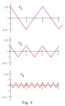
In the mid–1800s, the German mathematician Karl Weierstrass surprised and even shocked the mathematical world by creating a function which was continuous everywhere but differentiable nowhere - a function whose graph was everywhere connected and everywhere bent! He used techniques we have not investigated yet, but we can start to see how such a function could be built. 

Start with a function $f_1$ (Fig. 4) which zigzags between the values $+1/2$ and $–1/2$ and has a "corner" at each integer. This starting function $f_1$ is continuous everywhere and is differentiable everywhere except at the integers. Next create a list of functions $f_{2}, f_{3}, f_{4}, \ldots$, each of which is a lot shorter but with many more "corners" than the previous ones. For example, we might make $\mathrm{f}_{2}$ zigzag between the values $+1 / 4$ and $-1 / 4$ and have "corners" at $\pm 1 / 2, \pm 3 / 2$, $\pm 5 / 2$, etc., and $\mathrm{f}_{3}$ zigzag between $+1 / 9$ and $-1 / 9$ and have "corners" at $\pm 1 / 3$, $\pm 2 / 3, \pm 4 / 3$, etc. If we add $\mathrm{f}_{1}$ and $\mathrm{f}_{2}$, we get a continuous function (since the sum of two continuous functions is continuous) which will have corners at $0, \pm 1 / 2, \pm 1$, $\pm 3 / 2, \ldots$ If we then add $f_{3}$ to the previous sum, we get a new continuous function with even more corners. If we continue adding the functions in our list "indefinitely", the final result will be a continuous function which is differentiable nowhere.

We haven't developed enough mathematics here to precisely describe what it means to add an infinite number of functions together or to verify that the resulting function is nowhere differentiable, but we will. You can at least start to imagine what a strange, totally "bent" function it must be. 

Until Weierstrass created his "everywhere continuous, nowhere differentiable" function, most mathematicians thought a continuous function could only be "bad" in a few places, and Weierstrass' function was (and is) considered "pathological", a great example of how bad something can be. The mathematician Hermite expressed a reaction shared by many when they first encounter Weierstrass' function: 

"I turn away with fright and horror from this lamentable evil of functions which do not have derivatives".

IMPORTANT RESULTS

Power Rule For Functions: $\quad D\left(f^{n}(x)\right)=n \cdot f^{n-1}(x) \cdot D(f(x))$

Derivatives of the Trigonometric Functions:

$\begin{align*} \begin{array}{lll} \mathbf{D}(\sin (\mathrm{x}))=\cos (\mathrm{x}) & \mathrm{D}(\tan (\mathrm{x}))=\sec ^{2}(\mathrm{x}) & \mathrm{D}(\sec (\mathrm{x}))=\sec (\mathrm{x}) \tan (\mathrm{x}) \\ \mathbf{D}(\cos (\mathrm{x}))=-\sin (\mathrm{x}) & \mathrm{D}(\cot (\mathrm{x}))=-\csc ^{2}(\mathrm{x}) & \mathrm{D}(\csc (\mathrm{x}))=-\csc (\mathrm{x}) \cot (\mathrm{x}) \end{array} \end{align*}$

Derivatives of the Exponential Function: $\quad D\left(e^{x}\right)=e^{x}$

Practice 1: The pattern is $\mathbf{D}\left(\mathrm{f}^{\mathrm{n}}(\mathrm{x})\right)=\mathrm{n} \mathrm{f}^{\mathrm{n}-1}(\mathrm{x}) \cdot \mathbf{D}(\mathbf{f}(\mathbf{x})) . \mathbf{D}\left(\mathrm{f}^{5}\right)=5 \mathrm{f}^{4} \mathbf{D}(\mathbf{f})$ and $\mathbf{D}\left(\mathrm{f}^{13}\right)=13 \mathrm{f}^{12} \mathbf{D}(\mathbf{f})$

Practice 2: $\quad \frac{\mathrm{d}}{\mathrm{dx}}\left(2 \mathrm{x}^{5}-\pi\right)^{2}=2\left(2 \mathrm{x}^{5}-\pi\right)^{1} \mathrm{D}\left(2 \mathrm{x}^{5}-\pi\right)=2\left(2 \mathrm{x}^{5}-\pi\right)^{1}\left(10 \mathrm{x}^{4}\right)=40 \mathrm{x}^{9}-20 \pi \mathrm{x}^{4}$

$\begin{align*} \begin{aligned} &D\left(\left(x+7 x^{2}\right)^{1 / 2}\right)=\frac{1}{2}\left(x+7 x^{2}\right)^{-1 / 2} D\left(x+7 x^{2}\right)=\frac{1+14 x}{2 \sqrt{x+7 x^{2}}} \\ &D\left((\cos (x))^{4}\right)=4(\cos (x))^{3} D(\cos (x))=4(\cos (x))^{3}(-\sin (x))=-4 \cos ^{3}(x) \sin (x) \end{aligned} \end{align*}$

Practice 3:

$\begin{align*} \begin{aligned} &D\left(\frac{\cos (x)}{\sin (x)}\right)=\frac{\sin (x) D(\cos (x))-\cos (x) D(\sin (x))}{(\sin (x))^{2}} \\ &=\frac{\sin (x)(-\sin (x))-\cos (x)(\cos (x))}{\sin ^{2}(x)}=\frac{-\left(\sin ^{2}(x)+\cos ^{2}(x)\right)}{\sin ^{2}(x)}=\frac{-1}{\sin ^{2}(x)}=-\csc ^{2}(x) \end{aligned} \end{align*}$

Practice 4:

$\begin{align*} \begin{aligned} \mathbf{D}(\csc (x))=D\left(\frac{1}{\sin (x)}\right) &=\frac{\sin (x) D(1)-1 \mathbf{D}(\sin (x))}{\sin ^{2}(x)} \\ &=\frac{\sin (x)(0)-\cos (\mathbf{x})}{\sin ^{2}(x)}=-\frac{\cos (x)}{\sin (x)} \frac{1}{\sin (x)}=-\cot (x) \csc (x) \end{aligned} \end{align*}$

Practice 5: $\quad \mathbf{D}\left(x^{5} \cdot \tan (x)\right)=x^{5} D(\tan (x))+\tan (x) D\left(x^{5}\right)=x^{5} \sec ^{2}(x)+\tan (x)\left(5 x^{4}\right)$

$\begin{align*} \begin{aligned} &\frac{\mathbf{d}}{\mathrm{dt}}\left(\frac{\sec (\mathrm{t})}{\mathrm{t}}\right)=\frac{\mathrm{t} \mathbf{D}(\sec (\mathrm{t}))-\sec (\mathrm{t}) \mathbf{D}(\mathrm{t})}{\mathrm{t}^{2}}=\frac{\mathrm{t} \cdot \sec (\mathrm{t}) \cdot \tan (\mathrm{t})-\sec (\mathrm{t})}{\mathrm{t}^{2}} \\ &\begin{array}{l} \mathrm{D}\left((\cot (\mathrm{x})-\mathrm{x})^{1 / 2}\right) & =\frac{1}{2}(\cot (\mathrm{x})-\mathrm{x})^{-1 / 2} \mathrm{D}(\cot (\mathrm{x})-\mathrm{x}) \\ & =\frac{1}{2}(\cot (\mathrm{x})-\mathrm{x})^{-1 / 2}\left(-\csc ^{2}(\mathrm{x})-1\right)=\frac{-\csc ^{2}(\mathrm{x})-1}{2 \sqrt{\cot (\mathrm{x})-\mathrm{x}}} \end{array} \end{aligned} \end{align*}$

Practice 6:

Practice 7: $\quad D\left(x^{3} e^{x}\right)=x^{3} D\left(e^{x}\right)+e^{x} D\left(x^{3}\right)=x^{3}\left(e^{x}\right)+e^{x}\left(3 x^{2}\right)=x^{2} \cdot e^{x} \cdot(x+3)$

$\begin{align*}\begin{aligned}&D\left(\left(e^{x}\right)^{3}\right)=3\left(e^{x}\right)^{2} D\left(e^{x}\right)=3\left(e^{x}\right)^{2}\left(e^{x}\right)=3 e^{2 x} \cdot e^{x}=3 \mathrm{e}^{3 x} \end{aligned}\end{align*}$ or

$D\left(\left(e^{x}\right)^{3}\right)=D\left(e^{3 x}\right)=e^{3 x} D(3 x)=3 \mathbf{e}^{3 x}$

Practice 8: 

$\begin{array}{l|l|l}\mathrm{f}(\mathrm{x})=3 \mathrm{x}^{7} & \mathrm{f}(\mathrm{x})=\sin (\mathrm{x}) & \mathrm{f}(\mathrm{x})=\mathrm{x} \cdot \cos (\mathrm{x}) \\\mathrm{f}^{\prime}(\mathrm{x})=21 \mathrm{x}^{6} & \mathrm{f}^{\prime}(\mathrm{x})=\cos (\mathrm{x}) & \mathrm{f}^{\prime}(\mathrm{x})=-\mathrm{x} \cdot \sin (\mathrm{x})+\cos (\mathrm{x}) \\\mathrm{f}^{\prime \prime}(\mathrm{x})=126 \mathrm{x}^{5} & \mathrm{f}^{\prime \prime}(\mathrm{x})=-\sin (\mathrm{x}) & \mathrm{f}^{\prime \prime}(\mathrm{x})=-\mathrm{x} \cdot \cos (\mathrm{x})-2 \sin (\mathrm{x}) \\\mathrm{f}^{\prime \prime \prime}(\mathrm{x})=630 \mathrm{x}^{4} & \mathrm{f}^{\prime \prime \prime}(\mathrm{x})=-\cos (\mathrm{x}) & \mathrm{f}^{\prime \prime \prime}(\mathrm{x})=\mathrm{x} \cdot \sin (\mathrm{x})-3 \cos (\mathrm{x})\end{array}$