
Use the VLOOKUP function to search for data in vertical columns and the HLOOKUP function to search for data in horizontal rows.
Read these two sections on the VLOOKUP and HLOOKUP functions. The input for lookup functions is complicated, and you must be precise. Pay close attention to Tables 3.10 and 3.11, which detail the inputs for the two functions. Also, note the Skills Refreshers, which review the steps for entering the functions in Microsoft Excel.
Lookup functions are typically used to search for and display data in other worksheets or workbooks. The two lookup functions we will use in our personal investment portfolio example are the VLOOKUP and HLOOKUP functions.
The VLOOKUP function is typically used to access and display data in another worksheet or workbook. The function can also be used to access and display data located in the same worksheet. This is a very powerful and versatile function because it eliminates the need to copy or recreate existing data in other worksheets or workbooks. It is called a VLOOKUP function because it will search vertically down the first column of a range of cells to find a lookup value.
This process is very similar to statistical IF functions. You will recall that these functions used criteria to select cells from a range used in the mathematical output. The VLOOKUP function performs the same process. However, instead of selecting multiple cells from a range, the function only looks for one specific cell location. Once the function finds the specific cell location, it will display the contents of that cell location or another cell location in the range. Before using the VLOOKUP function in the personal investment portfolio workbook, it is strongly recommended that you carefully read the definitions for the function arguments listed in Table 1.
| Argument | Definition |
|---|---|
| Lookup_value | This argument is typically defined with a cell location, number, or text. Text data must be enclosed in quotation marks for this argument. The function will search for the criteria entered into this argument in the first column of the range used to define the Table_array argument. For example, if the word Hat is used to define this argument, the function will search for the word Hat in the first column of the range used to define the Table_array argument. |
| Table_array | Range of cells that contain data you wish the VLOOKUP function to search through (Lookup_value) and display. This cell range must contain the criteria used to define the Lookup_value in the first column. For example, if the range A2:D15 defines this argument, the criteria used to define the Lookup_value argument must exist in Column A. |
| Col_index_num | This is the column index number argument. It is defined with the number of columns to the right of the first column in the range used to define the Table_array argument that contains the data you wish to display. For example, suppose the data you wish the function to display is contained in Column C. If the range used to define the Table_array argument is A2:D15, then the column index number will be 3. Counting the columns to the right of the first column in this range, Column A would be 1, Column B would be 2, and Column C would be 3. It is important to remember to count the first column in the table array range as 1. |
| [Range_lookup] | This argument is defined with either the word TRUE or the word FALSE. When this argument is defined with the word FALSE, the function will look for an exact match to the criteria used to define the Lookup_value
argument in the first column of the table array range.
It is important to note the function will search the entire range to
find a match. If this argument is defined with the word TRUE, the function will look for a value that
is an exact match or the closest match that is less than
the lookup value. For example, if the lookup value is 80 and the
highest value in the first column of the table array range is 78, the
function will consider 78 a match
for the number 80. However, if the lookup value is 80 and the lowest number in the first column of the table array range is 85, the function will produce an error. This is because the number 80 and any value less than 80 do not exist in the first column of the table array range. It is important to note that if you define this argument with the word TRUE, the data in the table array range must be sorted in ascending order. This is because the function will stop searching for a match once the value in the first column exceeds the lookup value. If the data in the table array range is not sorted, the function can either produce an error code or display an erroneous result. This argument is in brackets because if it is not defined, it will automatically be defined with the word TRUE. |
Using a TRUE Range Lookup for VLOOKUP and HLOOKUP
If you are defining the Range_lookup argument with the word TRUE for either the VLOOKUP or HLOOKUP function, the range used to define the Table_array argument must be sorted in ascending order. For the VLOOKUP function, the table array range must be sorted from smallest to largest or from A to Z based on the values in the first column. For the HLOOKUP function, the table array range must be sorted from left to right based on the values in the first row, from smallest to largest or A to Z.
Descriptions for several investments are included in the workbook in the Investment List worksheet, as shown in Figure 1. The VLOOKUP function will be used to search for a specific symbol in Column A of the Investment List worksheet and display the description for that symbol located in Column B. The following steps explain how to accomplish this:
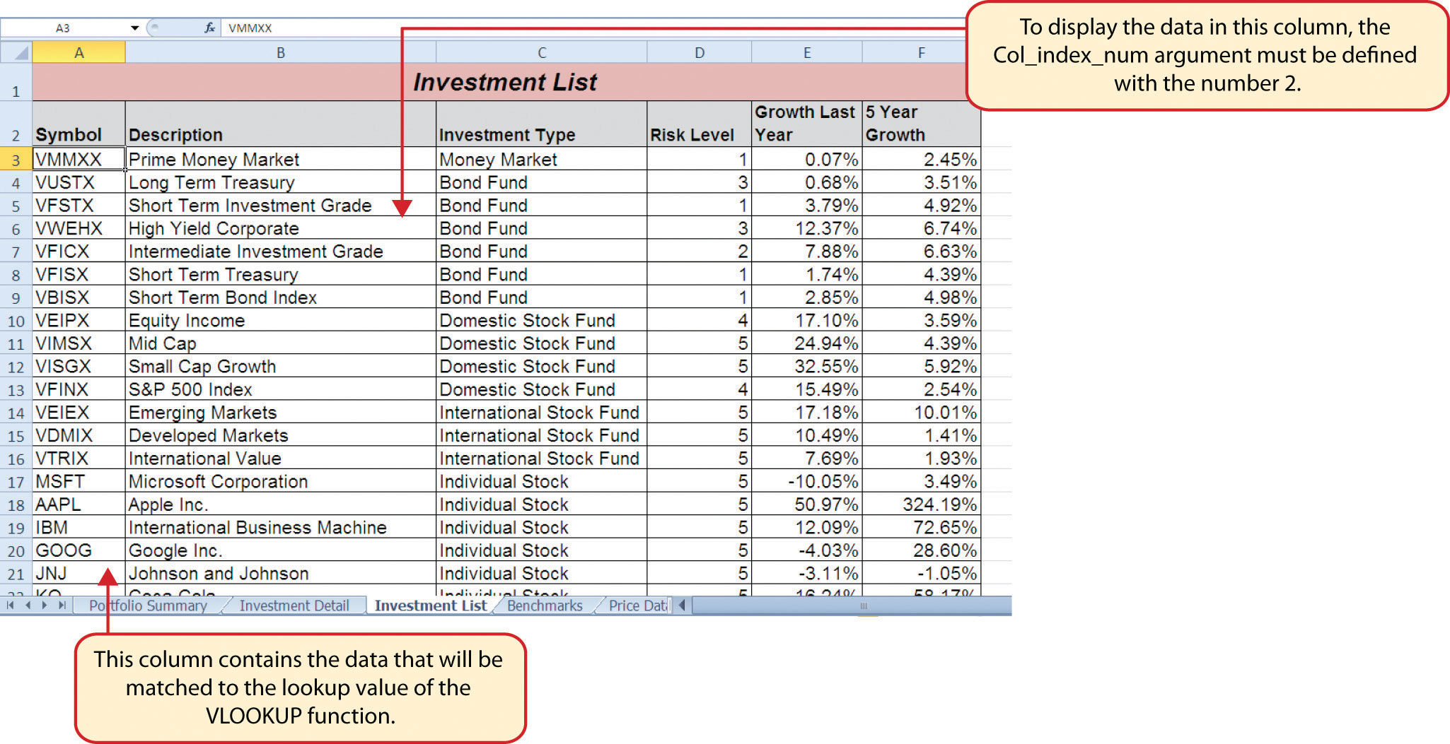
Figure 1 Investment List Worksheet
Figure 2 shows
the completed Function Arguments dialog box for the VLOOKUP function.
Notice that the Range_lookup argument is defined with the word FALSE.
This will direct the function to search for an exact match to the
lookup value and will also direct the function to search the entire
first column of the table array range. Finally, it is important to note
the absolute reference on the table array
range. This will prevent the table array range from changing when
the function is pasted into other cell locations.
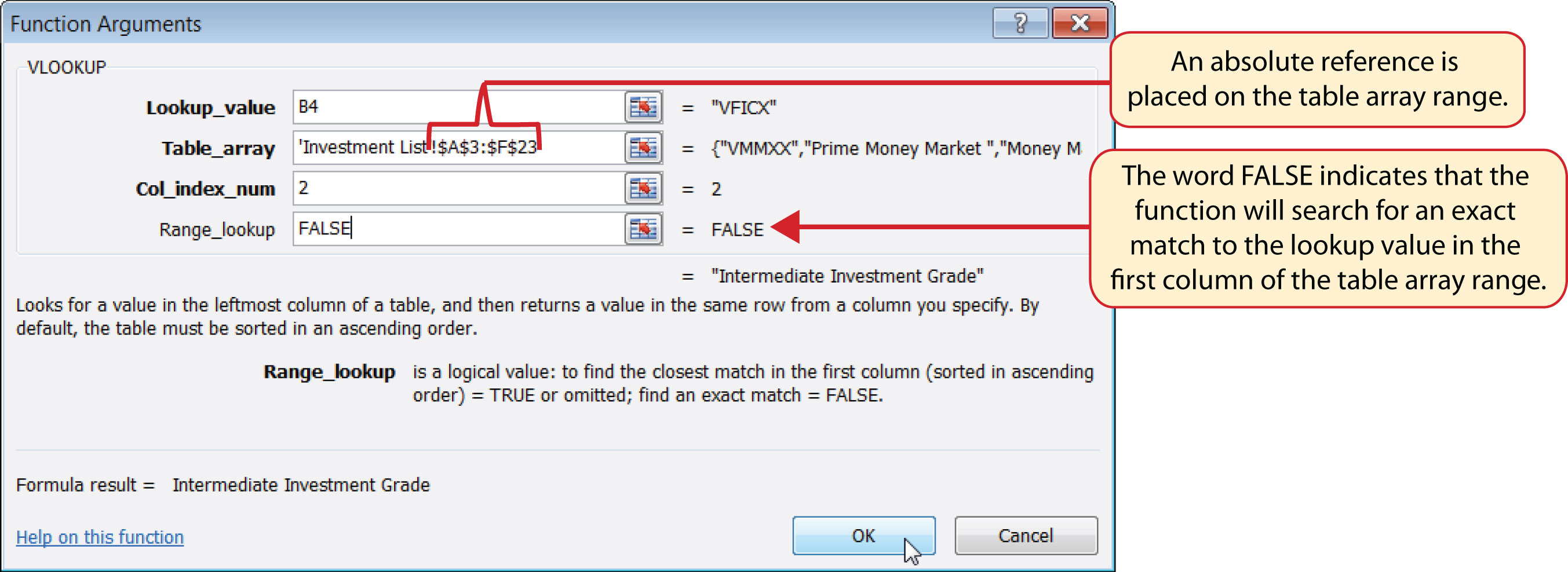
Figure 2 Completed Function Arguments Dialog Box for the VLOOKUP Function
Figure 3 shows the results of the VLOOKUP function in the Investment Detail worksheet. The function searches for each symbol in Column B
of the
Investment Detail worksheet in Column A of the Investment List
worksheet. When the function finds a match, it will display whatever is
in the cell location, two columns to the right, or Column B, in the Investment List worksheet. For example, the symbol VDMIX, which is in cell B8 on the Investment Detail worksheet (see Figure 3), is also in cell A15 on the Investment List worksheet (see Figure 1). As a result, the function displays whatever is in cell B15 on the Investment List worksheet, which is the description "Developed Markets."
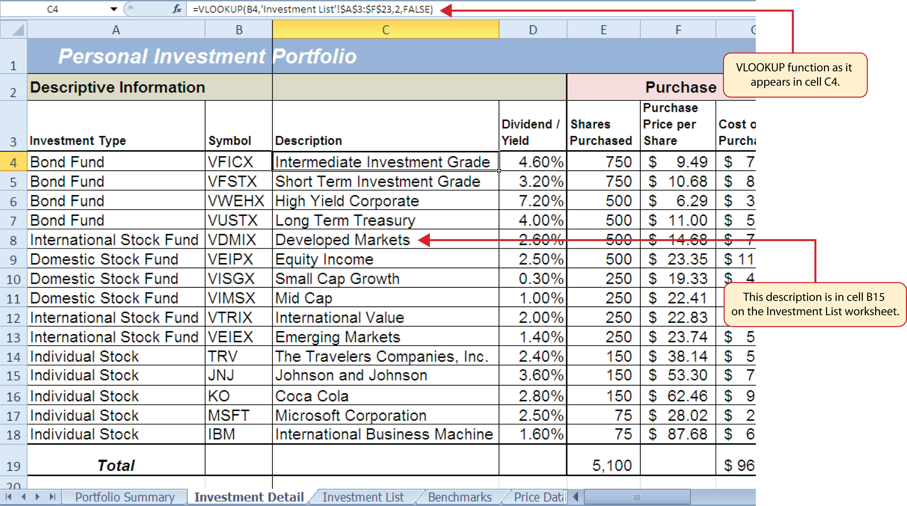
Figure 3 Results of the VLOOKUP Function in the Investment Detail Worksheet
Absolute References on the Table Array Range for the VLOOKUP and HLOOKUP Functions
If you are copying and pasting a VLOOKUP or HLOOKUP function, you will most likely need to place an absolute reference on the range used to define the Table_array argument. The table array range will change because of relative referencing once the function is pasted to new cell locations. This may result in an error output for either the VLOOKUP or HLOOKUP function. This is because the function will not be able to find the lookup value since the range has been adjusted. If you are defining the Range_lookup argument with the word TRUE, an adjustment in the table array range may result in an erroneous output.
Type an equal sign (=).
The HLOOKUP function serves the same purpose as the VLOOKUP function. The HLOOKUP function can display data from another worksheet or workbook. However, instead of searching for the lookup value vertically down the first column of the table array range, the HLOOKUP function searches horizontally across the first row of the table array range. When the function finds a match for the lookup value, it will display the contents in a cell location based on a row index number. This number designates how many rows the function should display below the first row of the table array range.
Table 2 provides a definition for each argument of the HLOOKUP function. It is best to review the definitions of these arguments carefully before using the function.
| Argument | Definition |
|---|---|
| Lookup_value | This argument is typically defined with a cell location, number, or text. Text data for this argument must be enclosed in quotation marks. The function will search for the criteria entered into this argument in the first row of the range used to define the Table_array argument. For example, if the word Hat is used to define this argument, the function will search for the word Hat in the first row of the range used to define the Table_array argument. |
| Table_array | Range of cells that contain data you wish the HLOOKUP function to search through (Lookup_value) and display. This cell range must contain the criteria used to define the Lookup_value in the first row. For example, if the range A2:D15 defines this argument, the criteria used to define the Lookup_value argument must exist in Row 2. |
| Row_index_num | This is the row index number argument. It is defined with the number of rows below the first row in the range used to define the Table_array argument that contains the data you wish to display. For example, suppose the data you wish the function to display is contained in Row 5. If the range used to define the Table_array argument is A2:D15, then the column index number will be 4. Counting the rows below the first row in this range, Row 2 would be 1, Row 3 would be 2, Row 4 would be 3, and Row 5 would be 4. It is important to remember to count the first row in the table array range as 1. |
| [Range_lookup] | This argument is defined with either the word TRUE or the word FALSE. When this argument is defined with the word FALSE, the function will look for an exact match to the criteria used to define the Lookup_value
argument in the first row of the table array range. It
is important to note the function will search the entire range to find a
match. If this argument is defined with the word TRUE, the function will look for a value that is
an exact match or the closest match that is less than the lookup value. For example, if the lookup value is 80 and the highest value in the first row of the table array range is 78, the function will consider 78 a match for the number 80. However, if the lookup value is 80 and the lowest number in the first row of the table array range is 85, the function will produce an error. This is because the number 80 and any value less than 80 do not exist in the first row of the table array range. It is important to note that if you define this argument with the word TRUE, the data in the table array range must be sorted based on the values in the first row in ascending order from left to right. This is because the function will stop searching for a match once the value in the first row exceeds the lookup value. If the table array range data is not sorted, the function can either produce an error code or display an erroneous result. This argument is in brackets because if it is not defined, it will automatically be defined with the word TRUE. |
The HLOOKUP function will be used on the Portfolio Summary worksheet to display the benchmark growth rates in the range G4:G7. A benchmark is a value that can be used as a standard point of comparison. The Benchmarks
worksheet contains growth rates at different year intervals for the
benchmarks that will be used to compare the performance for each
investment type (see Figure 4).
For this workbook, we
will compare the growth rates for each investment type to the
5-year average growth rate for the benchmark categories listed in the
range H4:H7.
The following steps explain how to construct the HLOOKUP
function to display the five-year benchmark
values in the Portfolio Summary worksheet:
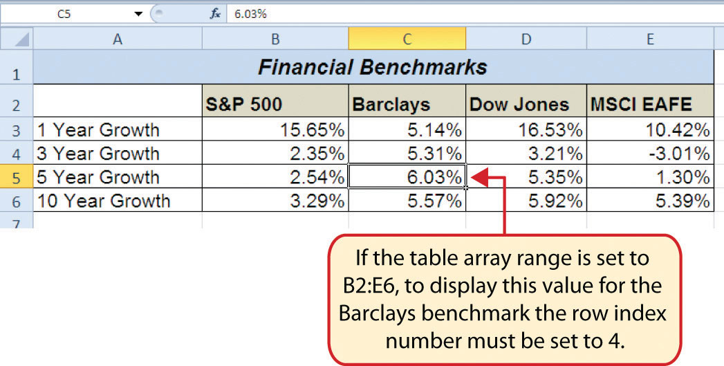
Figure 4 Benchmarks Worksheet
Figure 5 shows
the completed Function Arguments dialog box for the HLOOKUP function.
The row index number 4 indicates that the function will display the
contents
of the cell location in the fourth row of the table array range.
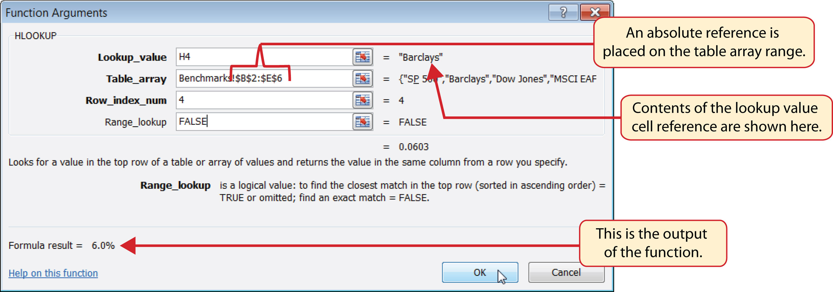
Figure 5 Completed Function Arguments Dialog Box for the HLOOKUP Function
Figure 6 shows
the output of the HLOOKUP function. Notice that the output of the
function in cell G4 is 6.0%. This is because the lookup value was
defined with the entry in cell H4, the Barclays index. Looking at Figure 4,
if you count the first row of the table array range as Row 1, the value
6.03% is the fourth row in the Barclays column. Since the values in
Column G on the Portfolio Summary worksheet are set to 1 decimal place, the value is displayed as 6.0%.
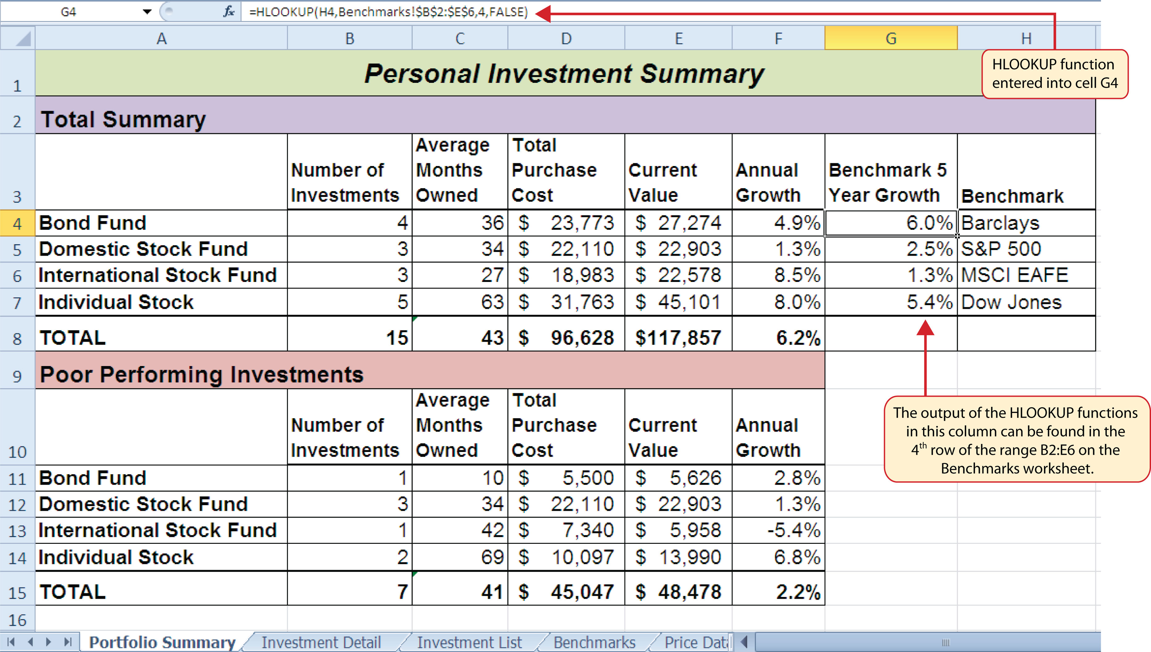
Figure 6 Completed Portfolio Summary Worksheet
#N/A and #REF! Errors with Lookup Functions
If you receive the #N/A error code when using the VLOOKUP or HLOOKUP function, it indicates that Excel cannot find the lookup value in the table array range. Check that the lookup value exists in the first column for the VLOOKUP, or the first row for the HLOOKUP, in the range used to define the Table_array argument. You may also see this error code if you copy and paste the function and forget to put an absolute reference on the range used to define the Table_array argument. The #REF! error code indicates that the column index number or row index number exceeds the number of columns or rows in the range used to define the Table_array argument.
 This text was adapted by Saylor Academy under
a Creative Commons Attribution-NonCommercial-ShareAlike 3.0 License without attribution as requested by the work's original creator or licensor.
This text was adapted by Saylor Academy under
a Creative Commons Attribution-NonCommercial-ShareAlike 3.0 License without attribution as requested by the work's original creator or licensor.